
14.4: Transformers
- Page ID
- 53027

\( \newcommand{\vecs}[1]{\overset { \scriptstyle \rightharpoonup} {\mathbf{#1}} } \)
\( \newcommand{\vecd}[1]{\overset{-\!-\!\rightharpoonup}{\vphantom{a}\smash {#1}}} \)
\( \newcommand{\id}{\mathrm{id}}\) \( \newcommand{\Span}{\mathrm{span}}\)
( \newcommand{\kernel}{\mathrm{null}\,}\) \( \newcommand{\range}{\mathrm{range}\,}\)
\( \newcommand{\RealPart}{\mathrm{Re}}\) \( \newcommand{\ImaginaryPart}{\mathrm{Im}}\)
\( \newcommand{\Argument}{\mathrm{Arg}}\) \( \newcommand{\norm}[1]{\| #1 \|}\)
\( \newcommand{\inner}[2]{\langle #1, #2 \rangle}\)
\( \newcommand{\Span}{\mathrm{span}}\)
\( \newcommand{\id}{\mathrm{id}}\)
\( \newcommand{\Span}{\mathrm{span}}\)
\( \newcommand{\kernel}{\mathrm{null}\,}\)
\( \newcommand{\range}{\mathrm{range}\,}\)
\( \newcommand{\RealPart}{\mathrm{Re}}\)
\( \newcommand{\ImaginaryPart}{\mathrm{Im}}\)
\( \newcommand{\Argument}{\mathrm{Arg}}\)
\( \newcommand{\norm}[1]{\| #1 \|}\)
\( \newcommand{\inner}[2]{\langle #1, #2 \rangle}\)
\( \newcommand{\Span}{\mathrm{span}}\) \( \newcommand{\AA}{\unicode[.8,0]{x212B}}\)
\( \newcommand{\vectorA}[1]{\vec{#1}} % arrow\)
\( \newcommand{\vectorAt}[1]{\vec{\text{#1}}} % arrow\)
\( \newcommand{\vectorB}[1]{\overset { \scriptstyle \rightharpoonup} {\mathbf{#1}} } \)
\( \newcommand{\vectorC}[1]{\textbf{#1}} \)
\( \newcommand{\vectorD}[1]{\overrightarrow{#1}} \)
\( \newcommand{\vectorDt}[1]{\overrightarrow{\text{#1}}} \)
\( \newcommand{\vectE}[1]{\overset{-\!-\!\rightharpoonup}{\vphantom{a}\smash{\mathbf {#1}}}} \)
\( \newcommand{\vecs}[1]{\overset { \scriptstyle \rightharpoonup} {\mathbf{#1}} } \)
\( \newcommand{\vecd}[1]{\overset{-\!-\!\rightharpoonup}{\vphantom{a}\smash {#1}}} \)
\(\newcommand{\avec}{\mathbf a}\) \(\newcommand{\bvec}{\mathbf b}\) \(\newcommand{\cvec}{\mathbf c}\) \(\newcommand{\dvec}{\mathbf d}\) \(\newcommand{\dtil}{\widetilde{\mathbf d}}\) \(\newcommand{\evec}{\mathbf e}\) \(\newcommand{\fvec}{\mathbf f}\) \(\newcommand{\nvec}{\mathbf n}\) \(\newcommand{\pvec}{\mathbf p}\) \(\newcommand{\qvec}{\mathbf q}\) \(\newcommand{\svec}{\mathbf s}\) \(\newcommand{\tvec}{\mathbf t}\) \(\newcommand{\uvec}{\mathbf u}\) \(\newcommand{\vvec}{\mathbf v}\) \(\newcommand{\wvec}{\mathbf w}\) \(\newcommand{\xvec}{\mathbf x}\) \(\newcommand{\yvec}{\mathbf y}\) \(\newcommand{\zvec}{\mathbf z}\) \(\newcommand{\rvec}{\mathbf r}\) \(\newcommand{\mvec}{\mathbf m}\) \(\newcommand{\zerovec}{\mathbf 0}\) \(\newcommand{\onevec}{\mathbf 1}\) \(\newcommand{\real}{\mathbb R}\) \(\newcommand{\twovec}[2]{\left[\begin{array}{r}#1 \\ #2 \end{array}\right]}\) \(\newcommand{\ctwovec}[2]{\left[\begin{array}{c}#1 \\ #2 \end{array}\right]}\) \(\newcommand{\threevec}[3]{\left[\begin{array}{r}#1 \\ #2 \\ #3 \end{array}\right]}\) \(\newcommand{\cthreevec}[3]{\left[\begin{array}{c}#1 \\ #2 \\ #3 \end{array}\right]}\) \(\newcommand{\fourvec}[4]{\left[\begin{array}{r}#1 \\ #2 \\ #3 \\ #4 \end{array}\right]}\) \(\newcommand{\cfourvec}[4]{\left[\begin{array}{c}#1 \\ #2 \\ #3 \\ #4 \end{array}\right]}\) \(\newcommand{\fivevec}[5]{\left[\begin{array}{r}#1 \\ #2 \\ #3 \\ #4 \\ #5 \\ \end{array}\right]}\) \(\newcommand{\cfivevec}[5]{\left[\begin{array}{c}#1 \\ #2 \\ #3 \\ #4 \\ #5 \\ \end{array}\right]}\) \(\newcommand{\mattwo}[4]{\left[\begin{array}{rr}#1 \amp #2 \\ #3 \amp #4 \\ \end{array}\right]}\) \(\newcommand{\laspan}[1]{\text{Span}\{#1\}}\) \(\newcommand{\bcal}{\cal B}\) \(\newcommand{\ccal}{\cal C}\) \(\newcommand{\scal}{\cal S}\) \(\newcommand{\wcal}{\cal W}\) \(\newcommand{\ecal}{\cal E}\) \(\newcommand{\coords}[2]{\left\{#1\right\}_{#2}}\) \(\newcommand{\gray}[1]{\color{gray}{#1}}\) \(\newcommand{\lgray}[1]{\color{lightgray}{#1}}\) \(\newcommand{\rank}{\operatorname{rank}}\) \(\newcommand{\row}{\text{Row}}\) \(\newcommand{\col}{\text{Col}}\) \(\renewcommand{\row}{\text{Row}}\) \(\newcommand{\nul}{\text{Nul}}\) \(\newcommand{\var}{\text{Var}}\) \(\newcommand{\corr}{\text{corr}}\) \(\newcommand{\len}[1]{\left|#1\right|}\) \(\newcommand{\bbar}{\overline{\bvec}}\) \(\newcommand{\bhat}{\widehat{\bvec}}\) \(\newcommand{\bperp}{\bvec^\perp}\) \(\newcommand{\xhat}{\widehat{\xvec}}\) \(\newcommand{\vhat}{\widehat{\vvec}}\) \(\newcommand{\uhat}{\widehat{\uvec}}\) \(\newcommand{\what}{\widehat{\wvec}}\) \(\newcommand{\Sighat}{\widehat{\Sigma}}\) \(\newcommand{\lt}{<}\) \(\newcommand{\gt}{>}\) \(\newcommand{\amp}{&}\) \(\definecolor{fillinmathshade}{gray}{0.9}\)Transformers have been in wide use in the electrical industry for over a century. Beginning with Michael Faraday and working through a sequence of scientists and inventors, the fundamentals of modern transformer design had been established by the late 1800s.
Transformer have three basic uses:
- Voltage scaling.
- Isolation.
- Impedance matching.
Transformers range from very small units used in communications systems up to large power distribution units many times the size of an adult human. A couple of transformers typical of the type used in consumer electronics devices is shown in Figure 10.4.1 . These devices are designed to handle standard residential AC input voltages (120 volts in North America, 220 to 240 volts in much of the remainder of the planet) and feeding circuits that demand perhaps 10 to 30 watts of power. The unit on the left is designed to be mounted directly onto a printed circuit board while the unit on the right is designed for chassis mount.
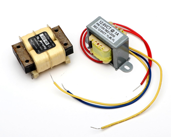
Figure 10.4.1 : Transformers suitable for consumer electronics devices. The unit on the left features four separate coils for enhanced flexibility.
In contrast, Figure 10.4.2 shows pole mounted transformers used to reduce typical North American residential distribution lines (in the vicinity of 15 kV) down to home voltage (120 volts). These transformers are capable of delivering 1000 or more times as much power as the transformers of Figure 10.4.1 . The transformers in these figures by no means present the extremes. Transformers are available that are considerably smaller or larger than the ones pictured here.
Transformers exploit magnetic circuit theory for their operation, as illustrated previously in Example 10.3.6. In its most basic form, the device has two coils or windings; one for the input side (called the primary winding) and one for the output side (the secondary winding). It is possible to have multiple input and/or output windings. Such is the case for the transformer on the left side of Figure 10.4.1 ; it has two input primary coils and two secondary coils. This allows for a variety of interconnection options, as we shall see. A typical schematic symbol is shown in Figure 10.4.3 . This symbol is appropriate for the magnetic system of Figure 10.3.15 which featured two coils. The vertical lines in the symbol represent the magnetic core.
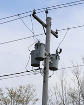
Figure 10.4.2 : A cluster of three residential power transformers.
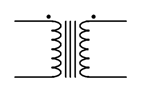
Figure 10.4.3 : Schematic symbol for a simple transformer.
Voltage Scaling and Isolation
A particularly important transformer parameter is the ratio of the number of turns on the primary coil \((N_P)\) to the number of turns on the secondary coil \((N_S)\). This is denoted \(N\), and referred to as the turns ratio.
\[N = \frac{N_P}{N_S} \label{10.13} \]
As the two windings are on the same core and ideally see the same flux, the voltage ratio of the primary to secondary will be equal to \(N\) for an ideal lossless transformer. Thus, if \(N=10\) and the primary voltage \((V_P)\) is 60 volts, the secondary voltage \((V_S)\) will be 6 volts. Thus:
\[V_S = \frac{V_P}{N} \label{10.14} \]
The primary and secondary appear as “\(NI\)” potentials in the magnetic circuit, therefore, the current will change inversely with \(N\). For example, if \(N=10\) and the primary current is 1 amp, the secondary current will be 10 amps. Thus:
\[I_S = N I_P \label{10.15} \]
It is important to note that the product of primary current and voltage must equal the product of secondary current and voltage for an ideal transformer. Such a device does not dissipate power but rather transforms it (hence the name).
\[V_S I_S = V_P I_P \label{10.16} \]
Real world devices will exhibit some loss due to finite winding wire resistance, nonideal behavior of the magnetic circuit and the like. Instead of a power dissipation rating, power transformers are given a VA (volt-amps) rating, typically thought of as secondary voltage times maximum secondary current. Transformers like the ones pictured in Figure 10.4.1 have ratings in the range of 10 to 30 VA. Generally, the higher the VA rating, the larger and heavier the transformer. On the other hand, applications using signal transformers in communications systems tend to focus on the turns ratio and not on the VA rating as the associated voltages and currents tend to be small. Their goal generally is to increase the amplitude of a signal voltage.
Also, because there is no direct electrical connection between the primary and secondary, the transformer may be used solely for isolation. This is a safety feature. If \(N=1\), then there is no change in the voltage being presented to the device, ideally.
A microphone feeds a small transformer which is used as the first stage of a preamplifier. The transformer has a primary winding of 50 turns and a secondary winding of 250 turns. Assuming an ideal transformer, determine the output voltage of the transformer if the signal from the microphone is 35 microvolts.
As this is an ideal transformer, the turns ratio indicates how much the input voltage is scaled. First we use Equation \ref{10.13} to determine the turns ratio.
\[N = \frac{N_P}{N_S} \nonumber \]
\[N = \frac{50}{250} \nonumber \]
\[N = 0.2 \nonumber \]
Now we use Equation \ref{10.14} to determine the secondary voltage.
\[V_S = \frac{V_P}{N} \nonumber \]
\[V_S = \frac{35 \mu V}{0.2} \nonumber \]
\[V_S = 175 \mu V \nonumber \]
Power applications will make use of \(N\) to scale the voltage in order to create a more appropriate or efficient level. If the voltage is brought down \((N>1)\), it is referred to as a step-down transformer. If \(N<1\), it is referred to as a step-up transformer. For example, a consumer electronics product may require a modest DC voltage for its operation, say 15 or 20 volts. To achieve this, the standard North American residential “wall” voltage of 120 volts may be reduced using a step-down transformer with \(N=5\). This would result in a secondary voltage of 24 volts that could then be rectified, filtered, and regulated to the desired DC level. Conversely, a step-up transformer could be used to create a much higher secondary potential (for example, in long distance power transmission to reduce \(I^2R\) losses). For some applications, split secondaries or multiple secondaries may be used. A center tap is relatively common and is used to divide the secondary into two equal voltage sections (e.g., a 24 volt center-tapped secondary would behave as two 12 volt secondaries in series). The schematic symbol for a transformer with a centertapped secondary is shown in Figure 10.4.4 .
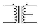
Figure 10.4.4 : Schematic symbol for a transformer with a centertapped secondary.
Multiple secondaries are also common and are more flexible than a center-tapped secondary. Multiple secondaries can be combined in series to increase the secondary voltage or combined in parallel to increase secondary current capacity (i.e, load current).
The power transformer shown in Figure 10.4.5 has turns ratio of 10. If the primary is connected to a 120 volt source and the secondary is connected in series with a 32 \(\Omega\) load resistor, determine the current through the load resistor. Assume this is an ideal transformer.
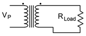
Figure 10.4.5 : Circuit for Example 10.4.2 .
The turns ratio indicates secondary voltage via Equation \ref{10.4}.
\[V_S = \frac{V_P}{N} \nonumber \]
\[V_S = \frac{120 V}{10} \nonumber \]
\[V_S = 12V \nonumber \]
Ohm's law can be used to find the secondary current.
\[I_S = \frac{V_S}{R_L} \nonumber \]
\[I_S = \frac{12V}{32 \Omega} \nonumber \]
\[I_S = 375mA \nonumber \]
As mentioned earlier, transformers work with AC voltages and currents. Unlike the consistent polarity of DC sources, AC (literally, Alternating Current) flips back and forth in voltage polarity and current direction. In order to determine the phase relationship between the primary and secondary, transformers use “dot notation”. The dot indicates the positive polarity of voltage. This is illustrated in the circuit of Figure 10.4.6 .
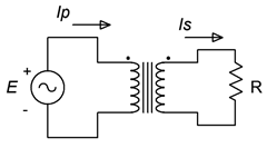
Figure 10.4.6 : Transformer dot convention.
On the primary side, the current flows into the dot and establishes the positive reference. In this case, the primary is seen as the load for the source, \(E\). On the secondary side, current flows out of the dot and also notates the positive reference because the secondary is seen as the source for the load, \(R\).
Impedance Matching
The third use of the transformer is impedance matching. Impedance is an AC phenomenon that consists of both resistance and reactance (an ohmic value associated with capacitors and inductors). The symbol for impedance is Z. Although impedance is measured in ohms, it differs from ordinary resistance in that it is a vector quantity and has a phase angle. For our present purposes, we can ignore this distinction.1
Because both the voltage and current are being scaled, the source's “view” of the load changes. The impedance seen by the source can be defined via Ohm's law as the voltage it produces divided by its output current.
\[Z_P = \frac{V_P}{I_P} \label{10.17} \]
From Equation \ref{10.14}, we know that \(V_P = V_S \cdot N\). Substituting this into Equation \ref{10.17} yields:
\[Z_P = \frac{V_S N}{I_P} \label{10.18} \]
From Equation \ref{10.15}, we know that \(I_P = I_S / N\). Substituting this into Equation \ref{10.18} yields:
\[Z_P = \frac{V_S N^2}{I_S} \label{10.19} \]
By definition,
\[Z_S = \frac{V_S}{I_S} \label{10.20} \]
Combining Equations \ref{10.19} and \ref{10.20} leaves us with:
\[Z_P = N^2 Z_S \label{10.21} \]
Thus, the impedance seen by the source is the secondary impedance times the square of the turns ratio. This is called the reflected impedance.
Assume that the transformer shown in Figure 10.4.6 has turns ratio of 5. If the primary is connected to an 20 volt source and the secondary is connected to an 8 \(\Omega\) load resistor, determine the primary current and the reflected impedance. Assume this is an ideal transformer.
First we'll use Equation \ref{10.21} to find the reflected impedance seen in the primary.
\[Z_P = N^2 Z_S \nonumber \]
\[Z_P = 5^2 \times 8 \Omega \nonumber \]
\[Z_P = 200 \Omega \nonumber \]
Ohm's law can be used to find the primary current.
\[I_P = \frac{V_P}{R_P} \nonumber \]
\[I_P = \frac{20V}{200\Omega} \nonumber \]
\[I_P = 100mA \nonumber \]
Here is where impedance matching comes in. In the preceding example, if the source, \(E\), had a large internal resistance compared to the load resistance, \(R\), and there was no transformer, there would be considerable loss in the system. For example, if the source impedance was 10 \(\Omega\) and it was directly connected to the 8 \(\Omega\) load without the transformer, the resulting voltage divider would cause a great deal of internal power dissipation in the source leading to inefficiency. On the other hand, in the given circuit with transformer, the source sees a reflected impedance of 200 \(\Omega\). The resulting voltage divider between 200 \(\Omega\) and the 10 \(\Omega\) internal resistance of the source will cause very little loss, yielding a much more efficient transfer.
References
1The concept of impedance is covered in great detail in the companion text, AC Electrical Circuit Analysis, another free OER title.