12.4: Memory Partitioning

Last updated
Save as PDF

Page ID: 82907

\( \newcommand{\vecs}[1]{\overset { \scriptstyle \rightharpoonup} {\mathbf{#1}} } \) \( \newcommand{\vecd}[1]{\overset{-\!-\!\rightharpoonup}{\vphantom{a}\smash {#1}}} \)\(\newcommand{\id}{\mathrm{id}}\) \( \newcommand{\Span}{\mathrm{span}}\) \( \newcommand{\kernel}{\mathrm{null}\,}\) \( \newcommand{\range}{\mathrm{range}\,}\) \( \newcommand{\RealPart}{\mathrm{Re}}\) \( \newcommand{\ImaginaryPart}{\mathrm{Im}}\) \( \newcommand{\Argument}{\mathrm{Arg}}\) \( \newcommand{\norm}[1]{\| #1 \|}\) \( \newcommand{\inner}[2]{\langle #1, #2 \rangle}\) \( \newcommand{\Span}{\mathrm{span}}\) \(\newcommand{\id}{\mathrm{id}}\) \( \newcommand{\Span}{\mathrm{span}}\) \( \newcommand{\kernel}{\mathrm{null}\,}\) \( \newcommand{\range}{\mathrm{range}\,}\) \( \newcommand{\RealPart}{\mathrm{Re}}\) \( \newcommand{\ImaginaryPart}{\mathrm{Im}}\) \( \newcommand{\Argument}{\mathrm{Arg}}\) \( \newcommand{\norm}[1]{\| #1 \|}\) \( \newcommand{\inner}[2]{\langle #1, #2 \rangle}\) \( \newcommand{\Span}{\mathrm{span}}\)\(\newcommand{\AA}{\unicode[.8,0]{x212B}}\)

Partition Allocation Methods in Memory Management

In the world of computer operating system, there are four common memory management techniques. They are:

Single contiguous allocation: Simplest allocation method used by MS-DOS. All memory (except some reserved for OS) is available to a process.
Partitioned allocation: Memory is divided into different blocks or partitions. Each process is allocated according to the requirement.
Paged memory management: Memory is divided into fixed-sized units called page frames, used in a virtual memory environment.
Segmented memory management: Memory is divided into different segments (a segment is a logical grouping of the process’ data or code).In this management, allocated memory doesn’t have to be contiguous.

Most of the operating systems (for example Windows and Linux) use segmentation with paging. A process is divided into segments and individual segments have pages.

In partition allocation, when there is more than one partition freely available to accommodate a process’s request, a partition must be selected. To choose a particular partition, a partition allocation method is needed. A partition allocation method is considered better if it avoids internal fragmentation.

When it is time to load a process into the main memory and if there is more than one free block of memory of sufficient size then the OS decides which free block to allocate.

There are different Placement Algorithm:

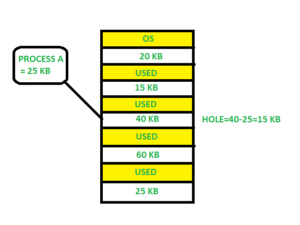
First Fit: In the first fit, the partition is allocated which is the first sufficient block from the top of main memory. It scans memory from the beginning and chooses the first available block that is large enough. Thus it allocates the first hole that is large enough.

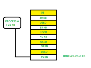
Figure \(\PageIndex{1}\): First Fit. ("First Fit" by deepakmkoshy, Geeks for Geeks is licensed under CC BY-SA 4.0)
Best Fit Allocate the process to the partition which is the first smallest sufficient partition among the free available partition. It searches the entire list of holes to find the smallest hole whose size is greater than or equal to the size of the process.

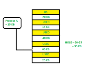
Figure \(\PageIndex{1}\): Best Fit. ("Best Fit" by deepakmkoshy, Geeks for Geeks is licensed under CC BY-SA 4.0)
Worst Fit Allocate the process to the partition which is the largest sufficient among the freely available partitions available in the main memory. It is opposite to the best-fit algorithm. It searches the entire list of holes to find the largest hole and allocate it to process.

Figure \(\PageIndex{1}\): Worst Fit. ("Worst Fit" by deepakmkoshy, Geeks for Geeks is licensed under CC BY-SA 4.0)
Next Fit: Next fit is similar to the first fit but it will search for the first sufficient partition from the last allocation point.

Adapted from:
"Partition Allocation Methods in Memory Management" by deepakmkoshy, Geeks for Geeks is licensed under CC BY-SA 4.0