7.3: Collision resolution

If two keys hash to the same index, the corresponding records cannot be stored in the same location. So, if it's already occupied, we must find another location to store the new record, and do it so that we can find it when we look it up later on.

To give an idea of the importance of a good collision resolution strategy, consider the following result, derived using the birthday paradox. Even if we assume that our hash function outputs random indices uniformly distributed over the array, and even for an array with 1 million entries, there is a 95% chance of at least one collision occurring before it contains 2500 records.

There are a number of collision resolution techniques, but the most popular are chaining and open addressing.

Chaining

Figure \(\PageIndex{1}\): Hash collision resolved by chaining. (Public Domain; via Wikimedia Commons)

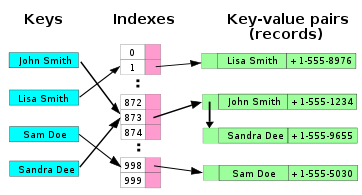
In the simplest chained hash table technique, each slot in the array references a linked list of inserted records that collide to the same slot. Insertion requires finding the correct slot, and appending to either end of the list in that slot; deletion requires searching the list and removal.

Chained hash tables have advantages over open addressed hash tables in that the removal operation is simple and resizing the table can be postponed for a much longer time because performance degrades more gracefully even when every slot is used. Indeed, many chaining hash tables may not require resizing at all since performance degradation is linear as the table fills. For example, a chaining hash table containing twice its recommended capacity of data would only be about twice as slow on average as the same table at its recommended capacity.

Chained hash tables inherit the disadvantages of linked lists. When storing small records, the overhead of the linked list can be significant. An additional disadvantage is that traversing a linked list has poor cache performance.

Alternative data structures can be used for chains instead of linked lists. By using a self-balancing tree, for example, the theoretical worst-case time of a hash table can be brought down to O(log n) rather than O(n). However, since each list is intended to be short, this approach is usually inefficient unless the hash table is designed to run at full capacity or there are unusually high collision rates, as might occur in input designed to cause collisions. Dynamic arrays can also be used to decrease space overhead and improve cache performance when records are small.

Some chaining implementations use an optimization where the first record of each chain is stored in the table. Although this can increase performance, it is generally not recommended: chaining tables with reasonable load factors contain a large proportion of empty slots, and the larger slot size causes them to waste large amounts of space.

Open addressing

Figure \(\PageIndex{2}\): Hash collision resolved by linear probing (interval=1). (Public Domain; via Wikimedia Commons)

Open addressing hash tables can store the records directly within the array. A hash collision is resolved by probing, or searching through alternate locations in the array (the probe sequence) until either the target record is found, or an unused array slot is found, which indicates that there is no such key in the table. Well known probe sequences include:

linear probing

in which the interval between probes is fixed—often at 1,

quadratic probing

in which the interval between probes increases linearly (hence, the indices are described by a quadratic function), and

double hashing

in which the interval between probes is fixed for each record but is computed by another hash function.

The main tradeoffs between these methods are that linear probing has the best cache performance but is most sensitive to clustering, while double hashing has poor cache performance but exhibits virtually no clustering; quadratic hashing falls in-between in both areas. Double hashing can also require more computation than other forms of probing. Some open addressing methods, such as last-come-first-served hashing and cuckoo hashing move existing keys around in the array to make room for the new key. This gives better maximum search times than the methods based on probing.

A critical influence on performance of an open addressing hash table is the load factor; that is, the proportion of the slots in the array that are used. As the load factor increases towards 100%, the number of probes that may be required to find or insert a given key rises dramatically. Once the table becomes full, probing algorithms may even fail to terminate. Even with good hash functions, load factors are normally limited to 80%. A poor hash function can exhibit poor performance even at very low load factors by generating significant clustering. What causes hash functions to cluster is not well understood, and it is easy to unintentionally write a hash function which causes severe clustering.

Example pseudocode

The following pseudocode is an implementation of an open addressing hash table with linear probing and single-slot stepping, a common approach that is effective if the hash function is good. Each of the lookup, set and remove functions use a common internal function findSlot to locate the array slot that either does or should contain a given key.

 record pair { key, value }
 var pair array slot[0..numSlots-1]
 
 function findSlot(key)
     i := hash(key) modulus numSlots
     loop
         if slot[i] is not occupied or slot[i].key = key
             return i
         i := (i + 1) modulus numSlots
 
 function lookup(key)
     i := findSlot(key)
     if slot[i] is occupied   // key is in table
         return slot[i].value
     else                     // key is not in table
         return not found     
 
 function set(key, value)
     i := findSlot(key)
     if slot[i].key = key
         // (Key already in table. Update value.)
         slot[i].value := value
     else
         // (Insert key and value in un-occupied slot.)
         // (But first, make sure insert won't overload the table)
         if the table is almost full
             rebuild the table larger (note 1)
             i := findSlot(key)
         slot[i].key   := key
         slot[i].value := value

Another example showing open addressing technique. Presented function is converting each part(4) of an Internet protocol address, where NOT is bitwise NOT, XOR is bitwise XOR, OR is bitwise OR, AND is bitwise AND and << and >> are shift-left and shift-right:

 // key_1,key_2,key_3,key_4 are following 3-digit numbers - parts of ip address xxx.xxx.xxx.xxx
 function ip(key parts)
     j := 1
     do
         key := (key_2 << 2)
         key := (key + (key_3 << 7))
         key := key + (j OR key_4 >> 2) * (key_4) * (j + key_1) XOR j
         key := key AND _prime_	// _prime_ is a prime number
         j := (j+1) 
     while collision
     return key

Note 1

Rebuilding the table requires allocating a larger array and recursively using the set operation to insert all the elements of the old array into the new larger array. It is common to increase the array size exponentially, for example by doubling the old array size.

 function remove(key)
     i := findSlot(key)
     if slot[i] is unoccupied
         return   // key is not in the table
     j := i
     loop
         j := (j+1) modulus numSlots
         if slot[j] is unoccupied
             exit loop
         k := hash(slot[j].key) modulus numSlots
         if (j > i and (k <= i or k > j)) or
            (j < i and (k <= i and k > j)) (note 2)
             slot[i] := slot[j]
             i := j
     mark slot[i] as unoccupied

Note 2

For all records in a cluster, there must be no vacant slots between their natural hash position and their current position (else lookups will terminate before finding the record). At this point in the pseudocode, i is a vacant slot that might be invalidating this property for subsequent records in the cluster. j is such as subsequent record. k is the raw hash where the record at j would naturally land in the hash table if there were no collisions. This test is asking if the record at j is invalidly positioned with respect to the required properties of a cluster now that i is vacant.

Another technique for removal is simply to mark the slot as deleted. However this eventually requires rebuilding the table simply to remove deleted records. The methods above provide O(1) updating and removal of existing records, with occasional rebuilding if the high water mark of the table size grows.

The O(1) remove method above is only possible in linearly probed hash tables with single-slot stepping. In the case where many records are to be deleted in one operation, marking the slots for deletion and later rebuilding may be more efficient.

Open addressing versus chaining

Chained hash tables have the following benefits over open addressing:

• They are simple to implement effectively and only require basic data structures.
• From the point of view of writing suitable hash functions, chained hash tables are insensitive to clustering, only requiring minimization of collisions. Open addressing depends upon better hash functions to avoid clustering. This is particularly important if novice programmers can add their own hash functions, but even experienced programmers can be caught out by unexpected clustering effects.
• They degrade in performance more gracefully. Although chains grow longer as the table fills, a chained hash table cannot "fill up" and does not exhibit the sudden increases in lookup times that occur in a near-full table with open addressing. (see right)
• If the hash table stores large records, about 5 or more words per record, chaining uses less memory than open addressing.
• If the hash table is sparse (that is, it has a big array with many free array slots), chaining uses less memory than open addressing even for small records of 2 to 4 words per record due to its external storage.

Figure \(\PageIndex{3}\): This graph compares the average number of cache misses required to lookup elements in tables with chaining and linear probing. As the table passes the 80%-full mark, linear probing's performance drastically degrades. (Public Domain; by Derrick Coetzee via Wikimedia Commons)

For small record sizes (a few words or less) the benefits of in-place open addressing compared to chaining are:

• They can be more space-efficient than chaining since they don't need to store any pointers or allocate any additional space outside the hash table. Simple linked lists require a word of overhead per element.
• Insertions avoid the time overhead of memory allocation, and can even be implemented in the absence of a memory allocator.
• Because it uses internal storage, open addressing avoids the extra indirection required for chaining's external storage. It also has better locality of reference, particularly with linear probing. With small record sizes, these factors can yield better performance than chaining, particularly for lookups.
• They can be easier to serialize, because they don't use pointers.

On the other hand, normal open addressing is a poor choice for large elements, since these elements fill entire cache lines (negating the cache advantage), and a large amount of space is wasted on large empty table slots. If the open addressing table only stores references to elements (external storage), it uses space comparable to chaining even for large records but loses its speed advantage.

Generally speaking, open addressing is better used for hash tables with small records that can be stored within the table (internal storage) and fit in a cache line. They are particularly suitable for elements of one word or less. In cases where the tables are expected to have high load factors, the records are large, or the data is variable-sized, chained hash tables often perform as well or better.

Ultimately, used sensibly any kind of hash table algorithm is usually fast enough; and the percentage of a calculation spent in hash table code is low. Memory usage is rarely considered excessive. Therefore, in most cases the differences between these algorithms is marginal, and other considerations typically come into play.

Coalesced hashing

A hybrid of chaining and open addressing, coalesced hashing links together chains of nodes within the table itself. Like open addressing, it achieves space usage and (somewhat diminished) cache advantages over chaining. Like chaining, it does not exhibit clustering effects; in fact, the table can be efficiently filled to a high density. Unlike chaining, it cannot have more elements than table slots.

Perfect hashing

If all of the keys that will be used are known ahead of time, and there are no more keys that can fit the hash table, perfect hashing can be used to create a perfect hash table, in which there will be no collisions. If minimal perfect hashing is used, every location in the hash table can be used as well.

Perfect hashing gives a hash table where the time to make a lookup is constant in the worst case. This is in contrast to chaining and open addressing methods, where the time for lookup is low on average, but may be arbitrarily large. There exist methods for maintaining a perfect hash function under insertions of keys, known as dynamic perfect hashing. A simpler alternative, that also gives worst case constant lookup time, is cuckoo hashing.

Probabilistic hashing

Perhaps the simplest solution to a collision is to replace the value that is already in the slot with the new value, or slightly less commonly, drop the record that is to be inserted. In later searches, this may result in a search not finding a record which has been inserted. This technique is particularly useful for implementing caching.

An even more space-efficient solution which is similar to this is use a bit array (an array of one-bit fields) for our table. Initially all bits are set to zero, and when we insert a key, we set the corresponding bit to one. False negatives cannot occur, but false positives can, since if the search finds a 1 bit, it will claim that the value was found, even if it was just another value that hashed into the same array slot by coincidence. In reality, such a hash table is merely a specific type of Bloom filter.