2.3: Modal dispersion

Modal dispersion is, essentially, the idea that each spatial mode has a different group velocity. This means that if you were to divide an input light pulse into two different spatial modes of a waveguide, the result would be that the two copies of the pulses would emerge from the waveguide at different times. This idealized picture indicates that it is possible to control which spatial modes of a waveguide are used. However, in general this is not true, and even if the coupling to the waveguide only put light into a single spatial mode, imperfections in the waveguide would scatter light into all other modes. So, in a communications system, the short sharp pulses of light required for high data rates spread out and overlap with each other. Ultimately, modal dispersion limits the product of distance and data rate: at short distances, high data rates are still possible, while over long distances only low data rates are possible.

Modal dispersion in a slab waveguide

In a first approximation, it is possible to understand modal dispersion simply be examining the path taken by a ray of light that propagates along the axis of a waveguide, compared to a ray of light that propagates at the critical angle, as shown in Figure \(\PageIndex{1}\). These two cases represent the highest and the lowest group velocity supported by the waveguide.

Figure \(\PageIndex{1}\): Shortest and longest paths through a waveguide with mirror-like reflections.

Here it is helpful to define the wavevector, \(k_0=\frac{2\pi}{\lambda_0}\) of a wave, which is modified by the material through which the wave travels: \(k = nk_0\). So far, we have only discussed the magnitude. The wavevector for the light paths in Figure \(\PageIndex{1}\) have a component along the axis of the waveguide \(k_z\) and a component that is transverse \(k_t\), which must vector sum to \(k\). The transverse wavevectors are given by

\[\begin{align} k_t &= nk_0\sin\gamma_m \\ k_t &= \frac{2\pi}{\lambda}\sin\gamma_m\\ k_t &= \frac{m\pi}{d} \label{eq:kTransverse} \end{align}\]

and the wavevectors along the axis are the wavevectors of the mode \(k_m\)

\[\begin{align} k^2_m &= k^2 - k_t^2\\ k^2_m &= k^2 - \frac{m^2\pi^2}{d^2} \\k^2_m &= \left(\frac{\omega}{c}\right)^2 - \frac{m^2\pi^2}{d^2} \label{eq:kAxis}\end{align}\]

Note that when \(m\) is large, \(k_m\) becomes imaginary, and the light cannot propagate in the waveguide. Note also, that for a given waveguide size, there is a lowest (angular) frequency that will propagate \(\omega_c = \frac{\pi c}{d}\). Equation \ref{eq:kAxis} is known as a dispersion relation and can be used to determine the the variation of group velocity with frequency and mode number, which, in turn, dictates the maximum data rate.

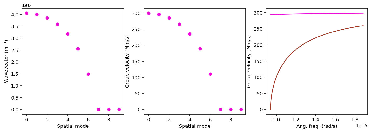
Figure \(\PageIndex{2}\) shows the change in \(k_m\) with mode number.

Figure \(\PageIndex{2}\): Modal wavevector with increasing mode number (left hand side), and corresponding group velocity (center) for a fixed frequency. Variation of group velocity with frequency for fundamental and 5th modes (right hand side).

The group velocity (the speed at which information is transferred) is given by \(v_g = \frac{\textrm{d}\omega}{\textrm{d} k}\) and can be obtained by taking the derivative of equation \ref{eq:kAxis}

\[\begin{align}2k_m\frac{\textrm{d} k_m}{\textrm{d}\omega} &= \frac{2\omega}{c^2}\\ \frac{k_mc^2}{\omega} &= \frac{\textrm{d}\omega}{\textrm{d}k_m}\\ \frac{\textrm{d}\omega}{\textrm{d}k_m} &= c\sqrt{1-\frac{m^2\omega_c^2}{\omega^2}} \label{eq:groupVelocity}\end{align}\]

Note that the group velocity for a given mode depends on both the waveguide dimensions and the frequency of the light wave. The variation of group velocity with mode number and frequency is shown in Figure \(\PageIndex{2}\).

Modal dispersion in "real" waveguides

In the discussion in Section \(\PageIndex{1}\), it was assumed that the entire wave traveled within the core of the waveguide (the reflections are mirror like), while in real waveguides, the spatial mode is distributed between the cladding and the core. The wavevector along the the axis of the waveguide is given by \(k_m = n_2k_0\cos\gamma_m\), where \(\gamma_c\geq\gamma_m \geq 0\). At \(\gamma_m = \gamma_c\), \(\cos\gamma_c = \frac{n_1}{n_2}\), so a substitution shows that \(k_m\) goes from \(n_1k_0\) to \(n_2k_0\). Or, put more qualitatively, the spatial modes go from looking like a wave traveling in the core material to looking like a wave traveling in the cladding material.

The dispersion relation for a dielectric slab waveguide is obtained from the self-consistency condition \(2k_td-2\phi_r = 2\pi m\), and can be expressed in the following way

\[\frac{\omega}{\omega_c} = \frac{\sqrt{n_2^2-n_1^2}}{\sqrt{n_2^2-n_{eff}^2}}\left(m + \frac{2}{\pi}\tan^{-1}\sqrt{\frac{n_{eff}^2-n_1^2}{n_2^2-n_{eff}^2}}\right) \label{eq:diSlDisp}\]

where \(n_{eff} = k_mc_0/\omega\) is the effective refractive index of the waveguide and \(\omega_c = \frac{2\pi c_o}{2d\textrm{NA}}\) is the angular frequency at which the mode cuts off.

Figure \(\PageIndex{3}\) shows the dispersion relation for different modes. Note that the traces track between the two light lines: one for the cladding (\(\omega = c_1k_m\)) and one for the core (\(\omega = c_2k_m\)). Tracking a mode from the moment the point at which it can begin to propagate (e.g., when the frequency is just above the cut off) onwards, notice that it starts near the light line for the cladding. In other words, near the cut off, the mode behaves as if it is propagating in the cladding, while at much higher frequencies the mode behaves as if it is propagating in the core material.

Figure \(\PageIndex{3}\): How the mode wavevector behaves with frequency.

The group velocity is obtained by taking the total derivative of equation \ref{eq:diSlDisp}, it is possible to obtain an approximate expression for the group velocity. Again, this is not derived in this text.

\[v_g = \frac{d\cot\theta + \Delta z}{\frac{d}{c_1}\csc\theta + \Delta\tau}\label{eq:gv}\]

where \(\Delta z\) and \(\Delta \tau\) take into account that total internal reflection is not instantaneous--the light penetrates slightly into the cladding material before returning. This can be through of as a slight displacement along the waveguide (\(\Delta z\)) that takes some amount of time (\(\Delta \tau\)). The upshot is that the group velocity of a mode at low frequency is close to that of the group velocity in the cladding (\(c_2\)), and as the frequency increases the group velocity reduces to that of the core (\(c_1\)).

Modal dispersion in optical fibers

For optical fibers with a large \(V\) number (recall that single mode operation occurs for \(V < 2.405\)), we have

\[\begin{align}k_{lm} &\approx \sqrt{n_2^2k_0^2 - \frac{2(l + 2m)^2\Delta}{M}}\\ k_{lm} &\approx n_2^2k_0^2 - \frac{(l + 2m)^2\Delta}{M}\label{eq:fibDisp}\end{align}\]

where \(\Delta =\frac{n_2^2-n_1^2}{2n_2^2}\approx \frac{n_2-n_1}{n_2}\ll 1\) is the refractive index contrast, and \(M\approx\frac{4V^2}{\pi^2}\) is the total number of modes supported by the fiber. The group velocity is obtained by find the derivative, \(\frac{\textrm{d}\omega}{\textrm{d}k_{lm}}\), of equation \ref{eq:fibDisp}, and can be shown to be approximately

\[v_{lm} \approx c_2\left(1 - \frac{(1 + 2m)^2\Delta}{M}\right)\]

Dispersion limits on communications

So far, we have a number of results showing that the group velocity is not the same for different optical modes in a waveguide or fiber. But, in a practical sense this is not hugely helpful. What we really want to know is that, if I have a pulse of duration \(\tau\) seconds, and I pass it through an optical fiber of length \(L\) meters, what will be the exit pulse duration?

For a highly multimode fiber (so large \(v\)), the minimum group velocity is \(v_{min} \approx c_2(1-\Delta)\) and the maximum group velocity is \(v_{max} = c_2\), where \(c_2\) is the speed of light in the core of the fiber. The transit times are \(t_{min} = \frac{L}{c_2(1-\Delta)}\) and \(t_{max} = L/c_2\) the pulse spreading is half the difference between these \(\delta t = \frac{L}{2c_2}\left(\frac{1}{(1-\Delta)} - 1\right)\). For \(\Delta\ll 1\) (which is typical for optical fibers) \(\frac{1}{1-\Delta}\approx 1 + \Delta\), so

\[\delta t \approx \frac{L\Delta}{2c_2}\label{eq:dt}\]

To generalize the result further, the dispersion of an optical fiber is usually expressed by the modal dispersion parameter, as time per unit length \(D_m = \frac{n_{co}\Delta}{2c_0}\), where, for clarity, \(c_2\), the speed of light, has been replaced with speed of light in the vacuum, \(c_0\), and the refractive index of the core, \(n_{co}\).

Note

Not all optical fibers use a step index as discussed above. There are also graded index fibers (GRIN fibers) that smoothly change the refractive index from the core to the cladding. GRIN fibers are always multimode, but the modal dispersion, \(D_m\) can be much less (ideally \(D_m = \frac{n_{co}\Delta^2}{4c_0}\). Recall that \(\Delta\ll 1\).

Limits to data rate

Now that it is possible to calculate how much a pulse will spread over a given distance, this provides two limits on the data rate. The first is that the light pulses spread from one time slot into the next causing low (or zero) intensity pulses to be mis-identified as bright pulses. The second is that the peak amplitude of the bright pulses becomes lower, so the contrast between low and high intensity reduces and increases the chance of a mis-identification. If we have a series of optical pulses in a fiber with an even duty cycle, the pulse spreading must be limited to about one quarter of the pulse time to ensure that the dark time-slots are still identified. So if the data rate is \(N\) b/s, then the bit time is \(1/N\) and \(\delta t \leq \frac{1}{4N}\). Substituting this result into equation \ref{eq:dt} gives \(NL \approx \frac{c_{0}}{2n_{co}\Delta}\) for a step index fiber. Note that for a given fiber (and ignoring material properties for now), everything on the right hand side is constant, so the data rate times the distance is a constant factor. Depending on an acceptable error rate and the modulation technique that is used, the factor 4 can change, changing the constant factor, but this is factors of two rather than orders of magnitude.

Example \(\PageIndex{1}\)

Two optical fibers, one a step index fiber with \(\Delta = 0.0034\) has a core refractive index of 1.46, and the second is a GRIN fiber with the same parameters what are the dispersion parameters for each fiber? Which is better?

In a communications application, the fiber must transport data over 100 m at a data rate of 10 Gb/s. Which, if either fiber can support the data rate?

Solution

The dispersion of the step fiber is \(D_m = \frac{n_{co}\Delta}{2c_0}\), where

• \(c_0 = 300\times 10^6\) m/s
• \(n_{co} = 1.46\)
• \(\Delta = 0.0034\)

putting these numbers in leads to \(D_m\) = 8.3 ns/km for the step index fiber

The dispersion for the GRIN fiber is \(D_m = \frac{n_{co}\Delta^2}{4c_0}\). Plugging the numbers gives \(D_m\) = 14 ps/km. The GRIN fiber is about 800 times better in terms of dispersion.

For \(N\) = 100 Gb/s and \(L=100\), we have \(NL\) = 10 Tm/s, while \(\frac{c_{0}}{2n_{co}\Delta}\) for the step index fiber is 0.03 Tm/s and for the GRIN fiber it is \(\frac{c_{0}}{n_{co}\Delta^2} =\) 18 Tm/s. Thus, we can conclude that the step index fiber cannot support the desired data rate over the required distance. The GRIN optical fiber does meet the requirements with room to spare.

Summary

Optical fibers and waveguides that support multiple modes are subject to modal dispersion. The dispersion spreads optical pulses, reducing their amplitude and causing communications pulses that are expected to fall within a certain time window to spread beyond their allotted window. If unaccounted for, modal dispersion will increase the error rate severely, and even prevent data transmission entirely. If the modal dispersion parameter \(D_m\) is known, modal dispersion can be accounted for in the system design.

Single mode devices are not effected by modal dispersion.