
2.5: Equilibrium Analysis for Concurrent Force Systems
- Page ID
- 102524

\( \newcommand{\vecs}[1]{\overset { \scriptstyle \rightharpoonup} {\mathbf{#1}} } \)
\( \newcommand{\vecd}[1]{\overset{-\!-\!\rightharpoonup}{\vphantom{a}\smash {#1}}} \)
\( \newcommand{\dsum}{\displaystyle\sum\limits} \)
\( \newcommand{\dint}{\displaystyle\int\limits} \)
\( \newcommand{\dlim}{\displaystyle\lim\limits} \)
\( \newcommand{\id}{\mathrm{id}}\) \( \newcommand{\Span}{\mathrm{span}}\)
( \newcommand{\kernel}{\mathrm{null}\,}\) \( \newcommand{\range}{\mathrm{range}\,}\)
\( \newcommand{\RealPart}{\mathrm{Re}}\) \( \newcommand{\ImaginaryPart}{\mathrm{Im}}\)
\( \newcommand{\Argument}{\mathrm{Arg}}\) \( \newcommand{\norm}[1]{\| #1 \|}\)
\( \newcommand{\inner}[2]{\langle #1, #2 \rangle}\)
\( \newcommand{\Span}{\mathrm{span}}\)
\( \newcommand{\id}{\mathrm{id}}\)
\( \newcommand{\Span}{\mathrm{span}}\)
\( \newcommand{\kernel}{\mathrm{null}\,}\)
\( \newcommand{\range}{\mathrm{range}\,}\)
\( \newcommand{\RealPart}{\mathrm{Re}}\)
\( \newcommand{\ImaginaryPart}{\mathrm{Im}}\)
\( \newcommand{\Argument}{\mathrm{Arg}}\)
\( \newcommand{\norm}[1]{\| #1 \|}\)
\( \newcommand{\inner}[2]{\langle #1, #2 \rangle}\)
\( \newcommand{\Span}{\mathrm{span}}\) \( \newcommand{\AA}{\unicode[.8,0]{x212B}}\)
\( \newcommand{\vectorA}[1]{\vec{#1}} % arrow\)
\( \newcommand{\vectorAt}[1]{\vec{\text{#1}}} % arrow\)
\( \newcommand{\vectorB}[1]{\overset { \scriptstyle \rightharpoonup} {\mathbf{#1}} } \)
\( \newcommand{\vectorC}[1]{\textbf{#1}} \)
\( \newcommand{\vectorD}[1]{\overrightarrow{#1}} \)
\( \newcommand{\vectorDt}[1]{\overrightarrow{\text{#1}}} \)
\( \newcommand{\vectE}[1]{\overset{-\!-\!\rightharpoonup}{\vphantom{a}\smash{\mathbf {#1}}}} \)
\( \newcommand{\vecs}[1]{\overset { \scriptstyle \rightharpoonup} {\mathbf{#1}} } \)
\(\newcommand{\longvect}{\overrightarrow}\)
\( \newcommand{\vecd}[1]{\overset{-\!-\!\rightharpoonup}{\vphantom{a}\smash {#1}}} \)
\(\newcommand{\avec}{\mathbf a}\) \(\newcommand{\bvec}{\mathbf b}\) \(\newcommand{\cvec}{\mathbf c}\) \(\newcommand{\dvec}{\mathbf d}\) \(\newcommand{\dtil}{\widetilde{\mathbf d}}\) \(\newcommand{\evec}{\mathbf e}\) \(\newcommand{\fvec}{\mathbf f}\) \(\newcommand{\nvec}{\mathbf n}\) \(\newcommand{\pvec}{\mathbf p}\) \(\newcommand{\qvec}{\mathbf q}\) \(\newcommand{\svec}{\mathbf s}\) \(\newcommand{\tvec}{\mathbf t}\) \(\newcommand{\uvec}{\mathbf u}\) \(\newcommand{\vvec}{\mathbf v}\) \(\newcommand{\wvec}{\mathbf w}\) \(\newcommand{\xvec}{\mathbf x}\) \(\newcommand{\yvec}{\mathbf y}\) \(\newcommand{\zvec}{\mathbf z}\) \(\newcommand{\rvec}{\mathbf r}\) \(\newcommand{\mvec}{\mathbf m}\) \(\newcommand{\zerovec}{\mathbf 0}\) \(\newcommand{\onevec}{\mathbf 1}\) \(\newcommand{\real}{\mathbb R}\) \(\newcommand{\twovec}[2]{\left[\begin{array}{r}#1 \\ #2 \end{array}\right]}\) \(\newcommand{\ctwovec}[2]{\left[\begin{array}{c}#1 \\ #2 \end{array}\right]}\) \(\newcommand{\threevec}[3]{\left[\begin{array}{r}#1 \\ #2 \\ #3 \end{array}\right]}\) \(\newcommand{\cthreevec}[3]{\left[\begin{array}{c}#1 \\ #2 \\ #3 \end{array}\right]}\) \(\newcommand{\fourvec}[4]{\left[\begin{array}{r}#1 \\ #2 \\ #3 \\ #4 \end{array}\right]}\) \(\newcommand{\cfourvec}[4]{\left[\begin{array}{c}#1 \\ #2 \\ #3 \\ #4 \end{array}\right]}\) \(\newcommand{\fivevec}[5]{\left[\begin{array}{r}#1 \\ #2 \\ #3 \\ #4 \\ #5 \\ \end{array}\right]}\) \(\newcommand{\cfivevec}[5]{\left[\begin{array}{c}#1 \\ #2 \\ #3 \\ #4 \\ #5 \\ \end{array}\right]}\) \(\newcommand{\mattwo}[4]{\left[\begin{array}{rr}#1 \amp #2 \\ #3 \amp #4 \\ \end{array}\right]}\) \(\newcommand{\laspan}[1]{\text{Span}\{#1\}}\) \(\newcommand{\bcal}{\cal B}\) \(\newcommand{\ccal}{\cal C}\) \(\newcommand{\scal}{\cal S}\) \(\newcommand{\wcal}{\cal W}\) \(\newcommand{\ecal}{\cal E}\) \(\newcommand{\coords}[2]{\left\{#1\right\}_{#2}}\) \(\newcommand{\gray}[1]{\color{gray}{#1}}\) \(\newcommand{\lgray}[1]{\color{lightgray}{#1}}\) \(\newcommand{\rank}{\operatorname{rank}}\) \(\newcommand{\row}{\text{Row}}\) \(\newcommand{\col}{\text{Col}}\) \(\renewcommand{\row}{\text{Row}}\) \(\newcommand{\nul}{\text{Nul}}\) \(\newcommand{\var}{\text{Var}}\) \(\newcommand{\corr}{\text{corr}}\) \(\newcommand{\len}[1]{\left|#1\right|}\) \(\newcommand{\bbar}{\overline{\bvec}}\) \(\newcommand{\bhat}{\widehat{\bvec}}\) \(\newcommand{\bperp}{\bvec^\perp}\) \(\newcommand{\xhat}{\widehat{\xvec}}\) \(\newcommand{\vhat}{\widehat{\vvec}}\) \(\newcommand{\uhat}{\widehat{\uvec}}\) \(\newcommand{\what}{\widehat{\wvec}}\) \(\newcommand{\Sighat}{\widehat{\Sigma}}\) \(\newcommand{\lt}{<}\) \(\newcommand{\gt}{>}\) \(\newcommand{\amp}{&}\) \(\definecolor{fillinmathshade}{gray}{0.9}\)If a body is in static equilibrium, then by definition that body is not accelerating. If we know that the body is not accelerating then we know that the sum of the forces acting on that body must be equal to zero. This is the basis for equilibrium analysis for a particle.
In order to solve for any unknowns in our sum of forces equation, we actually need to turn the one vector equation into a set of scalar equations. For two dimensional problems, we will split our one vector equation down into two scalar equations. We do this by summing up all the \(x\) components of the force vectors and setting them equal to zero in our first equation, and summing up all the \(y\) components of the force vectors and setting them equal to zero in our second equation.
\[ \sum \vec{F} \, = \, 0 \]
\[ \sum F_x \, = \, 0 \, ; \,\,\, \sum F_y \, = \, 0 \]
Once we have written out the equilibrium equations, we can solve the equations for any unknown forces.
Finding the Equilibrium Equations:
The first step in finding the equilibrium equations is to draw a free body diagram of the body being analyzed. This diagram should show all the known and unknown force vectors acting on the body. In the free body diagram, provide values for any of the know magnitudes or directions for the force vectors and provide variable names for any unknowns (either magnitudes or directions).
Next you will need to chose the \(x\), \(y\), and \(z\) axes. These axes do need to be perpendicular to one another, but they do not necessarily have to be horizontal or vertical. If you choose coordinate axes that line up with some of your force vectors you will simplify later analysis.
Once you have chosen axes, you need to break down all of the force vectors into components along the \(x\), \(y\) and \(z\) directions (see the vectors page in Appendix 1 if you need more guidance on this). Your first equation will be the sum of the magnitudes of the components in the \(x\) direction being equal to zero, the second equation will be the sum of the magnitudes of the components in the \(y\) direction being equal to zero, and the third (if you have a 3D problem) will be the sum of the magnitudes in the \(z\) direction being equal to zero. Collectively these are known as the equilibrium equations.
Once you have your equilibrium equations, you can solve them for unknowns using algebra. The number of unknowns that you will be able to solve for will be the number of equilibrium equations that you have. In instances where you have more unknowns than equations, the problem is known as a statically indeterminate problem and you will need additional information to solve for the given unknowns.
The diagram below shows a 3-lb box (Box A) sitting on top of a 5-lb box (box B). Determine the magnitude and direction of all the forces acting on box B.
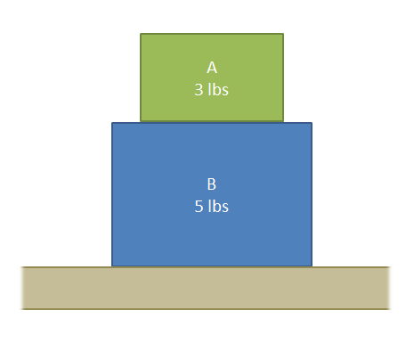 Figure \(\PageIndex{2}\): problem diagram for Example \(\PageIndex{1}\); two stacked boxes sitting on a flat surface.
- Solution
-
Video \(\PageIndex{2}\): Worked solution to example problem \(\PageIndex{1}\), provided by Dr. Jacob Moore. YouTube source: https://youtu.be/J54OZSitzzM. Video Transcript 2
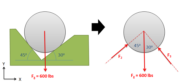
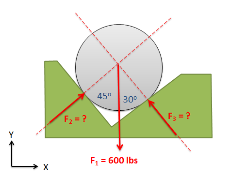
A 600-lb barrel rests in a trough as shown below. The barrel is supported by two normal forces (\(F_2\) and \(F_3\)). Determine the magnitude of both of these normal forces.
- Solution
-
Video \(\PageIndex{3}\): Worked solution to example problem \(\PageIndex{2}\), provided by Dr. Jacob Moore. YouTube source: https://youtu.be/qKhZvf55Bc0. Video Transcript 3
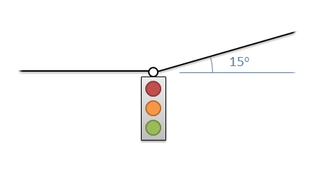
A 6-kg traffic light is supported by two cables as shown below. Find the tension in each of the cables supporting the traffic light.
- Solution
-
Video \(\PageIndex{4}\): Worked solution to example problem \(\PageIndex{3}\), provided by Dr. Jacob Moore. YouTube source: https://youtu.be/Oi2yDg1SmrI. Video Transcript 4
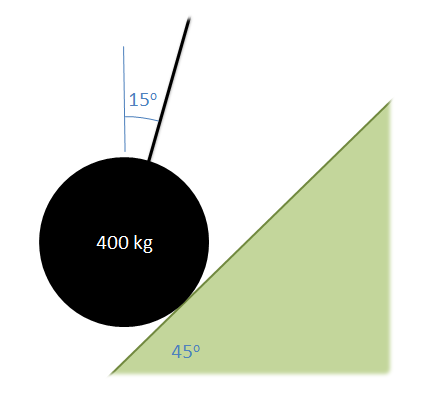
A 400-kg wrecking ball rests against a surface as shown below. Assuming the wrecking ball is currently in equilibrium, determine the tension force in the cable supporting the wrecking ball and the normal force that exists between the wrecking ball and the surface.
- Solution
-
Video \(\PageIndex{5}\): Worked solution to example problem \(\PageIndex{4}\), provided by Dr. Jacob Moore. YouTube source: https://youtu.be/gETMTfy5Sew. Video Transcript 5
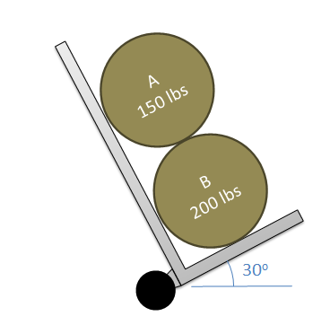
Barrels A and B are supported in a foot truck as seen below. Assuming the barrels are in equilibrium, determine all forces acting on barrel B.
- Solution
-
Video \(\PageIndex{6}\): Worked solution to example problem \(\PageIndex{5}\), provided by Dr. Jacob Moore. YouTube source: https://youtu.be/8DgrClhT4AM. Video Transcript 6
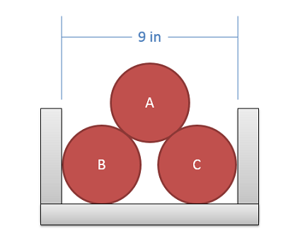
Three soda cans, each weighing 0.75 lbs and having a diameter of 4 inches, are stacked in a formation as shown below. Assuming no friction forces, determine the normal forces acting on can B.
- Solution
-
Video \(\PageIndex{7}\): Worked solution to example problem \(\PageIndex{6}\), provided by Dr. Jacob Moore. YouTube source: https://youtu.be/lAUahV7Mml4. Video Transcript 7