4.9: Recursive for Loops

By Carey A. Smith

A "recursive variable" in MATLAB is one whose updated value is a function of it's previous value. 

A "recursive for loop" is one in which the calculations for each iteration depend on the results of the previous iteration. It can have one or more recursive variables.

The Fibonacci sequence in section 4.6 is an example of a recursive for loop, because each term is the sum of the 2 previous values in the sequence.

A power sequence is another example of a recursive for loop.

Example \(\PageIndex{1}\) Power Sequence

% Initialize these variables:
n = 6;    % The number of terms in the sequence
A0 = 4; % The first value
r = 1/2;  % The ratio of successive terms
% Write a for loop that computes the terms in the sequence 
% which are computed with this expression:
%   A(k) = A0*r^k;
for k = 1:n
  A(k) = A0*r^k;
end
A % This diaplays all the values of the vector A

Solution

Add example text here.

.

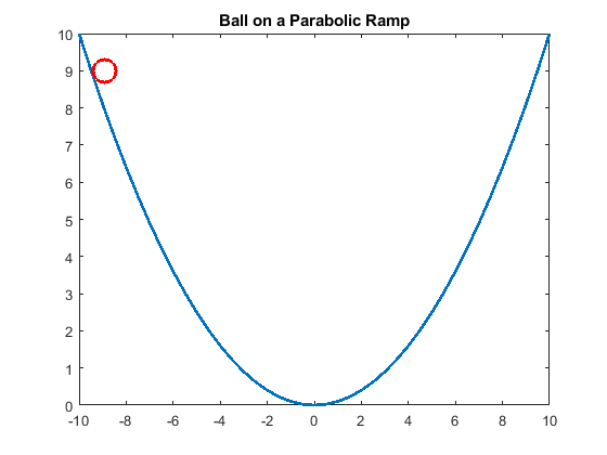
This is one example of a recursive loop. The height of the ball is the recursive variable.

Example \(\PageIndex{1}\)  Ball Rolling on a Parabola with Friction

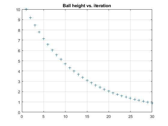
% A ball starts at height h1 on the ramp:

h1 = 10 % cm Initial height on the ramp

% Each time it rolls back and forth, it loses some energy due to friction

ff = 0.08 % The fraction of friction lost each iteration

% Use a for loop to compute the height on successive iterations.

% Let the number of iterations be:

n = 30

% Store the heights of each iteration in a vector.

% Initialize this vector to all zeros

h = zeros(1,n) % a row vector that is 8 long.

h(1) = h1

for k = 1:(n-1)

    h_loss = ff*h(k);

    h(k+1) = h(k) - h_loss;

end

%% Draw a parabolic ramp
x = -10:0.5:10;
y = (0.1)*x.^2;
figure;
plot(x,y,'LineWidth',2)

% Add a ball
bxc = -8.9; % ball center
byc = 9; % ball center
hold on;
plot(bxc, byc,'ro','MarkerSize',16,'LineWidth',2)
title('Ball on a Parabolic Ramp')

%% Plot the vector of heights with '+' markers

figure

plot(h, '+')

grid on

title('height vs, iteration')

ylim([0,h1])

Solution

Add example text here.

.

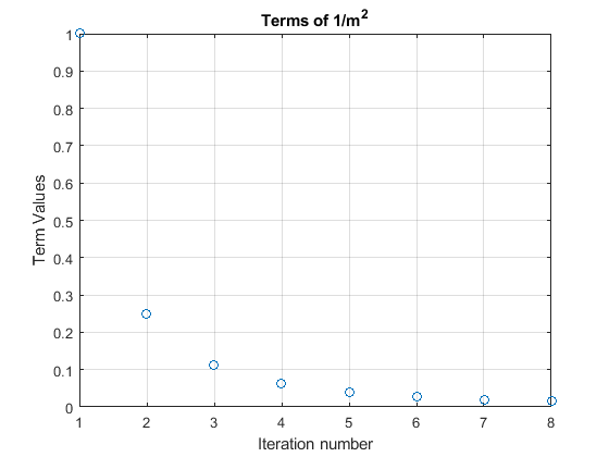
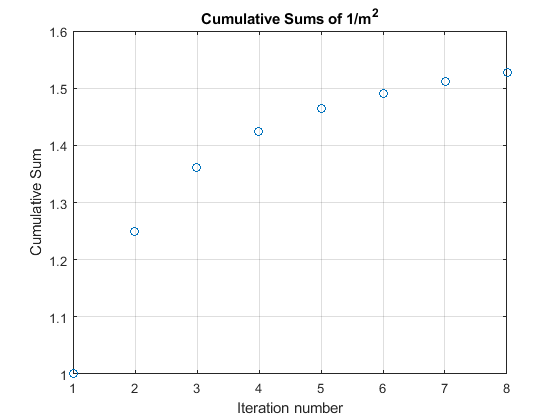
The summation of a series is an example of a recursive loop. The total is a recursive variable.

Example \(\PageIndex{2}\) Cumulative Sum Vector Plot

format compact; format short g; 
clear all; close all; clc;
%% Initialize the term and total vectors
term = zeros(1,8);    % Initialize the term vector
total = zeros(1,8);   % Initialize the total vector
term(1) = 1/1^2;
total(1)= term(1);
for m = 2:8
  term(m) = 1/m^2;
  total(m) = total(m-1) + term(m);
end
%% Display the final value
disp(['The final sum= ',num2str(total(end))])
% Display the last term
disp(['The last term= ',num2str(term(end))])

%% Plot the terms
figure;
plot(term,'o')
grid on;
title('Terms of 1/m^2')
xlabel('Iteration number')
ylabel('Term Values')

%% Plot the cumulative sums
figure;
plot(total,'o')
grid on;
title('Cumulative Sums of 1/m^2')
xlabel('Iteration number')
ylabel('Cumulative Sum')

Answer

.

.

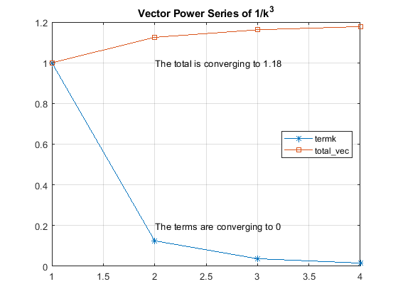
The following recursive sum example compares the code for a scalar total (the total is a single value) to the code for a vector total (the total vector includes the totals for each iteration).

When there are 2 data sets plotted on 1 figure, you can use the legend() function that identifies each data set, as shown in the following example.

It also shows the use of the text() function to place information on the figure. This is used in combination with the num2str() function to convert a computed value to a character string that can become part of a title or text, using concatenation of character strings.

Example \(\PageIndex{3}\) Scalar vs. Vector Sums

%% Scalar loop sum
n = 4; % n = the number of terms in the series
total_scalar = 0; % This total is updated on each iteration
for k = 1:n
    term = 1/k^3;
   % Sum the series using either of these 2 methods:
   % cum_sum(m) = cum_sum(m-1) + term(m);  % Method 1

   cum_sum_new = cum_sum(m-1) + term(m);  % Method 2

   cum_sum(m) = cum_sum_new;

    total_scalar = total_scalar + term;   % Method 1
    % Update total by adding the current term to the previous value of total.
    % Recall that "=" means assignment, not equality.

    total_new = total_scalar + term;   % Method 2
    total_scalar = total_new;
end
total_scalar % echo the final total
% total_scalar = 1.1777
% This is a scalar loop sum, because termk and total are single values which change on each iteration

%% Vector loop sum
n = 4; % n = the number of terms in the series
total_vec = zeros(1,n); % This total is updated on each iteration
% total_vec(k) will be the partial sum of the terms up thru the kth term.
% Initial the 1st term and the total:
k = 1;
termk(k) = 1/k^3;
total_vec(k) = termk(k);
for k = 2:n % Start with k=2, becuz the loop uses total_vec(k-1)
    termk(k) = 1/k^3;
    total_vec(k) = total_vec(k-1) + termk(k);
    % Update total by adding the current term to the previous value of total.
    % New value is total(k). Previous value is total(k-1)
    % Recall that "=" means assignment, not equality.
end
total_vec % Echo total_vec

%% Since termk and total_vec are vectors, we can plot them after the for loop.
kk = 1:n; % This is the x-axis vector
figure;
plot(kk, termk, '-*')
hold on;
plot(kk, total_vec, '-s')
grid on;
legend('termk','total\_vec','Location','East')
title('Vector Power Series of 1/k^3')

If you are using MATLAB, add this code:
  total_end = round(total_vector(end),2) % Round to 2 decimal places

If you are using Octave, add this code:

  total_end = total_vector(end)  % Don't round

text(2,1,['The total is converging to ',total_str]) % concatenate the words with the number
text(2,0.2,'The terms are converging to 0')

Solution

% total_scalar = 1.1777

% total_vec = 1 1.125 1.162 1.1777

 

.

. 

Population growth is another example of a recursive for loop.

Example \(\PageIndex{4}\) Population Growth of Chipmunks

Figure \(\PageIndex{i}\): https://commons.wikimedia.org/wiki/File:Chipmunk_in_PP_(93909).jpg
Creative Commons Attribution-Share Alike 4.0 International license.

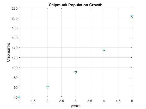
% Population growth of chipmunks
n = 5 % The number of years (iterations)
% Create this vector:
chipmunks = zeros(1,n);
% The population starts with 40 individuals, so set the 1st value = 40.
chipmunks(1) = 40;
% Assume that there are approximately equal numbers of males and females.

% Start a for loop that models the size of this population for 5 years.
% Let the for loop index be k; k will go from 1 to (n-1),
%  because it computes the population for year k+1, based on year k.

for k = 1:(n-1)
    % Inside the for loop do the following to update the number of chipmunks 
    %  for each for successive year:
    % Each year, on average, 40% of the chipmunks die, so compute:
    died = round(0.40*chipmunks(k)) % chipmunks(k) is the number at the beginning of year k.
    % The round() function makes sure that the result is an integer.
    % Subtract the number that died from the population.  
    %  Let the resulting number be called survivors.
    survivors = chipmunks(k) - died
    % Compute an average of 3 baby chipmunks for each pair of surviving chipmunks
    %  and round this value:
    babies = round(3*(survivors/2))
    % Add the babies to the surviving foxes 
    %  to get the new total population for the start of the next year:
  chipmunks(k+1) = survivors + babies
end % end the for loop

% After the loop end, open a new figure and plot the number of chipmunks each year.
% Use the ‘v’ marker for each data point.
figure
plot(chipmunks,'v')
  % (1 pt) Turn the grid on and add a title and axis labels:
grid on
title('Chipmunk Population Growth')
xlabel('years')
ylabel('Chipmunks')

Solution

Add example text here.

Many variations on the population growth example are possible.

Exercise \(\PageIndex{1}\) Modified Population Growth

Modify the chipmunk population growth example by changing the death rate and/or the birth rate, such that the number of chipmunks after 5 years is a value between 1.5 and 3 times the initial population.

This will require some trial and error.

Answer

Figure this out on your own.

. 

There is a potential problem that you must avoid. If you create a program that mistakenly calls itself, this creates an unintentional recursive infinite loop. It may only stop when the maximum number of recursive calls allowed by MATLAB/Octave is reached (about 500 calls) or if you kill the program either by closing MATLAB/Octave or keying Ctrl-C. When a student writes a script that calls itself, it is almost always a mistake. However, there are a very few valid, specialized functions that use recursive calls to themselves, such as code search for free memory to be allocated. Such code must have logic to end the self-calling recursion.

.