10.3: Linear and Polynomial Curve Data Fitting

Linear Data Fitting

Interpolation is appropriate when you have a limited amount of accurate data and want to estimate the value of a function between the given data points.

Linear data fitting is appropriate when you have data with random errors, but you believe that the relation between x & y should be approximately linear. In this case, you do not want to connect the data points with lines using interpolation. Rather you want to calculated the best-fit line to the data.This best-fit line will not go through each data point. Rather, it will be a straight line that minimizes the distance between the data points and the line. The approach finds a line that minimizes the sum of the squares of the differences between the data y-values and the y values predicted by y(k) = m*x(k) + b. This is know as the Least-Squares method. (For more information, you can read https://en.wikipedia.org/wiki/Least_squares.) Linear data fitting is also called "linear regression".)

For example, the physics formula relating voltage (V), current (I) and resistance (R) of an electrical component is:

V = I*R

You may want to estimate the resistance of a component by measuring the current through the component and the voltage across the positive and negative connections of the component.

Another example is that you have multiple factors affecting a measurement, but you want a linear approximation for the relation between 2 particular  variables.

The main functions for finding the linear approximation are polyfit() and polyval(). Assuming that your data are in vectors x and y, the steps are:

Step 1: Compute the coefficients using the polyfit() function:

coeffs=polyfit(x,y,1);

Step 2: Use the computed coefficients to compute the y values of the line at the x data points using the polyval() function.

>besty=coeffs(1)*x+coeffs(2);

This process is illustrated in the example below.

Example \(\PageIndex{1}\) Linear Fit for data with measurement errors

This example begins by creating linear data with radom errors.

x0 = 0:1:10;
y0 = 2*x0;
% Add measurement noise
y1 = y0 + 2*randn(size(y0))

One run of this code produced these y1 values:

y1 = [1.0759,  4.4454,  4.7333, 7.5520,  9.0903,  9.5448, 12.4408,  12.8191,  17.3326, 16.2794,  18.3967]

figure;   % Plot these data
hold on;
plot(x0,y1,'ko');
grid on;

% Step 1: Compute the coefficients using the polyfit() function:
coef1 = polyfit(x0,y1,1)

% coef1 = [1.6875    1.8999]
 

% Step 2: Use the computed coefficients to compute the y values of the line at the x data points using the polyval() function.
y2b = polyval(coef1,x0);

% Plot the best fit line on the same plat as the original data
plot(x0,y2b,'r--','LineWidth',2);
title('Linear Data Fit Example 1')

The plot shows that the line computed by the linear fit averages out most of the radom errors ("noise") in the original data.

Solution

Add example text here.

The next example shows a linear fit to data influenced by multiple factors.

Example \(\PageIndex{2}\) Linear Data Fitting for Vehicle Fuel Economy

This example computes a linear fit to fuel economy vs. vehicle weight.

In this example, fuel economy is the gallons of fuel used per 100 miles.

Factors that affect fuel efficiency include weight, size of the engine, the coefficient of drag, and the friction in all the moving parts, so we don't expect a line to be a perfect fit for fuel efficiency vs. weight. But, it is useful to see the trend between these 2 variables.

% Linear fit to car fuel economy. References for 2024 vehicles
% https://www.fueleconomy.gov/feg/Find...tion=sbsSelect
% https://www.chevrolet.com/

% Variables:
% w = weight
% mpg = miles per gallon
% gp100m = gallons/100 miles
%
% Trailblazer
w(1) = 3252;
mpg(1) =   30;
gp100m(1) = 100/mpg(1)

% Equinox
w(2) = 3512;
mpg(2) =   26;
gp100m(2) = 100/mpg(2)
 

% Malibu (2023)
w(3) = 3161;
mpg(3) =   30;
gp100m(3) = 100/mpg(3)

% Suburban
w(4) = 5723;
mpg(4) =   16;
gp100m(4) = 100/mpg(4)
 

% Tahoe
w(5) = 5580;
mpg(5) =   17;
gp100m(5) = 100/mpg(5)

% Chevrolet Camaro, 6-cyl, 3.6 L
w(6) = 3351;
mpg(6) = 22;
gp100m(6) = 100/mpg(6)

% Chevrolet Corvette Stingray
w(7) = 3366;
mpg(7) = 19;
gp100m(7) = 100/mpg(7)

% Chevrolet Trax 1.2 L
w(8) = 3000; % Approximate
mpg(8) = 30;
gp100m(8) = 100/mpg(8)

%% Plot
figure;
plot(w,gp100m,'o')
xlim([0,7000])
ylim([0,7])
grid on;

%% Linear fit
coeffs_eff = polyfit(w, gp100m, 1)
w2 = 2000 : 500: 7000;
eff_fit2 = polyval(coeffs_eff, w2);
hold on;
plot(w2, eff_fit2,'-r');
xlabel('Vehicle Weight')
ylabel('Gallons per 100 miles')
title('Fuel Efficiency vs. Vehicle Weight')

Solution

Add example text here.

.

 Polynomial Curve Fitting 

Sometimes the relation of the data is non-linear. In this case, a polynomial file is better than a linear fit.

The following example is from Troy Siemers (). 9.1: Curve Fitting by Troy Siemers is licensed CC BY-NC 3.0. Original source:

https://drive.google.com/file/d/0B2Pdg3LqVPNPLUhLbks0QzF5ZVhmWGp3YW5hYlVBd3RDN2x3/view?resourcekey=0-fbyowylmkO1jBbS2ehDP0g&usp=sharing.

First we show the data with a linear fit.

Example \(\PageIndex{2}\) Curve Fit to Non-Linear Data  

x=0:5;y=[12,10,9,6,2,0];

figure
plot(x,y,'o')

%% Compute a linear fit to the data
coeffs1 = polyfit(x,y,1);
% The command polyfit returns the matrix [-2.4857 12.7143]
% This is the slope and y-intercept of the line of best fit.
% Compute and plot the best-fit line
besty1  = coeffs1(1)*x+coeffs1(2);

% Plot the best-fit line on the same graph
hold on;
plot(x,besty1)

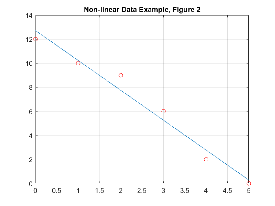
Looking closely at the data, we can see that it curves down. We can compute and plot 2nd-order and 5th-order curve fits.

coeffs2 = polyfit(x,y,2);
 

This time, we will use the function polyval(),  which is simpler for higher-order curves.

x2 = 0 : 0.25 : 5;
y2=polyval(coeffs2,x2);
plot(x2, y2, '+g','Linewidth',3)
title('Non-linear Data Example, 2nd Order Curve Fit')

We see that the 2nd-order curve fit is a somewhat better fit to the data.

We can also do a 5th-order fit to the data.

coeffs5 = polyfit(x,y,5)
y5 = polyval(coeffs5,x2);
plot(x2, y5, '*r')
title('Non-linear Data Example, 2nd and 5th-Order Curve Fits')

 

Since there are 6 data points, a 5th-order data fit goes through every every point. This might seem like a good thing, but it is likely bogus, unless we have a good reason to believe that the data really is 5th-order. This is known as "over fitting". A rule-of-thumb is that you should have at least 2*n data point for an nth-order curve fit. See these links for details, potential problems, and alternatives:

https://en.wikipedia.org/wiki/Curve_fitting

This Mathworks link explains the peril of extrapolation (plotting the curve for x-values beyond the range of the original data x-values.

https://www.mathworks.com/help/matlab/ref/polyfit.html

 

 

Solution

Add example text here.

 

Fitting by Transforming the Data

Sometimes physical data is measured data as a function of time.

This data in this example is temperature of water as a function of time. The water starts at 100 degrees C and cools off over time.

Both 2nd-order and 3rd-order polynomials are fitted to the data. Both fit well over the first 80 seconds of data. But the 2nd-order fit increases at the end, implying that the water started to get hotter, instead of continuing to cool off. So, the 3rd order curve makes more physical sense.

The nex section demonstate show a 5th-order polynomial curve fit to the data in section 10.3

Example \(\PageIndex{1}\) Polyvnomial Curve Fit of Water Temperature vs. Time

% Measured data for cooling of hot water vs. time
time1 = 0 : 10: 100;
temperature_t0 = 100 % degrees C
temp0 = temperature_t0*exp(-0.03*time1)
temperature_measured = [100, 70, 57, 40, 32, 20, 17, 12, 8, 6, 5]
figure;
plot(time1, temperature_measured,'sk');
grid on;
hold on;
% 2nd order fit
coeffs_temp2 = polyfit(time1, temperature_measured, 2)
time2 = 0 : 2: 100;
temp_fit2 = polyval(coeffs_temp2, time2);
plot(time2, temp_fit2,'+b');
% 3rd-order fit
coeffs_temp3 = polyfit(time1, temperature_measured, 3)
temp_fit3 = polyval(coeffs_temp3, time2);
plot(time2, temp_fit3,'*r');

title('Curve-fitting of Water Temperature Decay')

legend('Data', '2nd-order fit polynomial', '3rd Order fit')

Solution

The plot for this example is shown here:

 

.

Exponential Curve-Fitting

This section and the previous sections show how to do linear and polynomial curve-fitting. Sometimes we expect an exponential function to fit the data batter than a polynomial. An exponential curve is a better fit for many physical phenomena. Often the data can be transformed to be approximately linear. Then a linear fit can be computed and the result can then be transformed back to the original space as an exponential curve. The following is an example of how to do that.

Example \(\PageIndex{2}\) Exponential Curve Fit  

% Exponential Curve-Fit by Transforming the Data
% Measured data for cooling of hot water vs. time
time1 = 0 : 10: 100;
temperature_t0 = 100 % degrees C
temp0 = temperature_t0*exp(-0.03*time1)
temperature_measured = [100, 70, 57, 40, 32, 20, 17, 12, 8, 6, 5]
figure;
plot(time1, temperature_measured,'sk');
grid on;
hold on;
% We expect the temperature decay to be exponential
% By computing the natural logarithm, the data becomes linear:
log_temperature = log(temperature_measured);
% Linear fit to the logarithm of the data:
log_coeffs_temp1 = polyfit(time1, log_temperature, 1);
log_temp_fit1 = polyval(log_coeffs_temp1, time2);
figure;
plot(time1, log_temperature,'sk');
grid on;
hold on;
plot(time2, log_temp_fit1,'+b');
title('Linear-fit of the Logarithm of Water Temperature')
legend('Data', 'Linear fit')
% Transform back to original space
figure;
plot(time1, temperature_measured,'sk');
grid on;
hold on;
temp_logfit1 = exp(log_temp_fit1);
plot(time2, temp_logfit1,'+b');
% Convert linear fit to an exponential function
temp_fit1 = exp(log_coeffs_temp1(2))*exp(log_coeffs_temp1(1)*time2);
plot(time2, temp_fit1,'or');
title('Exponential Curve-Fit of Water Temperature Decay')
legend('Data', 'exp(1st-order fit)', 'exponential fit')

Solution

This plot shows that the exponential fitting process works.

 

 

 

.