
14.2: Plot 3D Surface and Contour Plots
- Page ID
- 85207

\( \newcommand{\vecs}[1]{\overset { \scriptstyle \rightharpoonup} {\mathbf{#1}} } \)
\( \newcommand{\vecd}[1]{\overset{-\!-\!\rightharpoonup}{\vphantom{a}\smash {#1}}} \)
\( \newcommand{\dsum}{\displaystyle\sum\limits} \)
\( \newcommand{\dint}{\displaystyle\int\limits} \)
\( \newcommand{\dlim}{\displaystyle\lim\limits} \)
\( \newcommand{\id}{\mathrm{id}}\) \( \newcommand{\Span}{\mathrm{span}}\)
( \newcommand{\kernel}{\mathrm{null}\,}\) \( \newcommand{\range}{\mathrm{range}\,}\)
\( \newcommand{\RealPart}{\mathrm{Re}}\) \( \newcommand{\ImaginaryPart}{\mathrm{Im}}\)
\( \newcommand{\Argument}{\mathrm{Arg}}\) \( \newcommand{\norm}[1]{\| #1 \|}\)
\( \newcommand{\inner}[2]{\langle #1, #2 \rangle}\)
\( \newcommand{\Span}{\mathrm{span}}\)
\( \newcommand{\id}{\mathrm{id}}\)
\( \newcommand{\Span}{\mathrm{span}}\)
\( \newcommand{\kernel}{\mathrm{null}\,}\)
\( \newcommand{\range}{\mathrm{range}\,}\)
\( \newcommand{\RealPart}{\mathrm{Re}}\)
\( \newcommand{\ImaginaryPart}{\mathrm{Im}}\)
\( \newcommand{\Argument}{\mathrm{Arg}}\)
\( \newcommand{\norm}[1]{\| #1 \|}\)
\( \newcommand{\inner}[2]{\langle #1, #2 \rangle}\)
\( \newcommand{\Span}{\mathrm{span}}\) \( \newcommand{\AA}{\unicode[.8,0]{x212B}}\)
\( \newcommand{\vectorA}[1]{\vec{#1}} % arrow\)
\( \newcommand{\vectorAt}[1]{\vec{\text{#1}}} % arrow\)
\( \newcommand{\vectorB}[1]{\overset { \scriptstyle \rightharpoonup} {\mathbf{#1}} } \)
\( \newcommand{\vectorC}[1]{\textbf{#1}} \)
\( \newcommand{\vectorD}[1]{\overrightarrow{#1}} \)
\( \newcommand{\vectorDt}[1]{\overrightarrow{\text{#1}}} \)
\( \newcommand{\vectE}[1]{\overset{-\!-\!\rightharpoonup}{\vphantom{a}\smash{\mathbf {#1}}}} \)
\( \newcommand{\vecs}[1]{\overset { \scriptstyle \rightharpoonup} {\mathbf{#1}} } \)
\(\newcommand{\longvect}{\overrightarrow}\)
\( \newcommand{\vecd}[1]{\overset{-\!-\!\rightharpoonup}{\vphantom{a}\smash {#1}}} \)
\(\newcommand{\avec}{\mathbf a}\) \(\newcommand{\bvec}{\mathbf b}\) \(\newcommand{\cvec}{\mathbf c}\) \(\newcommand{\dvec}{\mathbf d}\) \(\newcommand{\dtil}{\widetilde{\mathbf d}}\) \(\newcommand{\evec}{\mathbf e}\) \(\newcommand{\fvec}{\mathbf f}\) \(\newcommand{\nvec}{\mathbf n}\) \(\newcommand{\pvec}{\mathbf p}\) \(\newcommand{\qvec}{\mathbf q}\) \(\newcommand{\svec}{\mathbf s}\) \(\newcommand{\tvec}{\mathbf t}\) \(\newcommand{\uvec}{\mathbf u}\) \(\newcommand{\vvec}{\mathbf v}\) \(\newcommand{\wvec}{\mathbf w}\) \(\newcommand{\xvec}{\mathbf x}\) \(\newcommand{\yvec}{\mathbf y}\) \(\newcommand{\zvec}{\mathbf z}\) \(\newcommand{\rvec}{\mathbf r}\) \(\newcommand{\mvec}{\mathbf m}\) \(\newcommand{\zerovec}{\mathbf 0}\) \(\newcommand{\onevec}{\mathbf 1}\) \(\newcommand{\real}{\mathbb R}\) \(\newcommand{\twovec}[2]{\left[\begin{array}{r}#1 \\ #2 \end{array}\right]}\) \(\newcommand{\ctwovec}[2]{\left[\begin{array}{c}#1 \\ #2 \end{array}\right]}\) \(\newcommand{\threevec}[3]{\left[\begin{array}{r}#1 \\ #2 \\ #3 \end{array}\right]}\) \(\newcommand{\cthreevec}[3]{\left[\begin{array}{c}#1 \\ #2 \\ #3 \end{array}\right]}\) \(\newcommand{\fourvec}[4]{\left[\begin{array}{r}#1 \\ #2 \\ #3 \\ #4 \end{array}\right]}\) \(\newcommand{\cfourvec}[4]{\left[\begin{array}{c}#1 \\ #2 \\ #3 \\ #4 \end{array}\right]}\) \(\newcommand{\fivevec}[5]{\left[\begin{array}{r}#1 \\ #2 \\ #3 \\ #4 \\ #5 \\ \end{array}\right]}\) \(\newcommand{\cfivevec}[5]{\left[\begin{array}{c}#1 \\ #2 \\ #3 \\ #4 \\ #5 \\ \end{array}\right]}\) \(\newcommand{\mattwo}[4]{\left[\begin{array}{rr}#1 \amp #2 \\ #3 \amp #4 \\ \end{array}\right]}\) \(\newcommand{\laspan}[1]{\text{Span}\{#1\}}\) \(\newcommand{\bcal}{\cal B}\) \(\newcommand{\ccal}{\cal C}\) \(\newcommand{\scal}{\cal S}\) \(\newcommand{\wcal}{\cal W}\) \(\newcommand{\ecal}{\cal E}\) \(\newcommand{\coords}[2]{\left\{#1\right\}_{#2}}\) \(\newcommand{\gray}[1]{\color{gray}{#1}}\) \(\newcommand{\lgray}[1]{\color{lightgray}{#1}}\) \(\newcommand{\rank}{\operatorname{rank}}\) \(\newcommand{\row}{\text{Row}}\) \(\newcommand{\col}{\text{Col}}\) \(\renewcommand{\row}{\text{Row}}\) \(\newcommand{\nul}{\text{Nul}}\) \(\newcommand{\var}{\text{Var}}\) \(\newcommand{\corr}{\text{corr}}\) \(\newcommand{\len}[1]{\left|#1\right|}\) \(\newcommand{\bbar}{\overline{\bvec}}\) \(\newcommand{\bhat}{\widehat{\bvec}}\) \(\newcommand{\bperp}{\bvec^\perp}\) \(\newcommand{\xhat}{\widehat{\xvec}}\) \(\newcommand{\vhat}{\widehat{\vvec}}\) \(\newcommand{\uhat}{\widehat{\uvec}}\) \(\newcommand{\what}{\widehat{\wvec}}\) \(\newcommand{\Sighat}{\widehat{\Sigma}}\) \(\newcommand{\lt}{<}\) \(\newcommand{\gt}{>}\) \(\newcommand{\amp}{&}\) \(\definecolor{fillinmathshade}{gray}{0.9}\)By Carey A. Smith
meshgrid() function
Surface plots need 2-dimensional grids of x and y coordinates. These are made from 1-dimensional vectors of x and y coordinates using the meshgrid() function. The syntax of meshgrid() is:
[x2D, y2D] = meshgrid(x1D,y1D);
x1D = [0, 1, 2 ,3];
y1D = [0, 2, 4];
[x2D, y2D] = meshgrid(x1D,y1D)
Solution
x2D =
0 1 2 3
0 1 2 3
0 1 2 3
y2D =
0 0 0 0
2 2 2 2
4 4 4 4
As can be seen:
The x coordinates are repeated in all the rows.
The x coordinates are repeated in all the columns.
Watch this video about meshgrid. Note that the presenter uses lower case x & y for 1-dimensional values and upper case X & Y for 1-dimensional values. It is not good practice to use variables names that only differ by lower and upper case. Better is to use different name, like x1D, y1D and x2D, y2D. The important part is 0 to 4:20 minutes.
.
mesh() 3D Plot
The mesh() function creates a wire-frame 3-dimensional plot.
%% Create a 3D graph of r^2 = x^2 + y^2 over a grid of points
% 1. Set the x and y axis 1D vectors that define this rectangular grid:
x1D = -3 : 0.5 :3; % 1x13 vector
y1D = -2.5: 0.5 :2.5; % 1x11 vector
%% 2. Matlab's meshgrid() function uses these 1D vectors
% to create 2D arrays of x & y at each point of the rectangular grid.
[x2D, y2D] = meshgrid(x1D,y1D);
%% 3. Compute z(x,y) at each point in the grid.
z = x2D.^2 + 1*x2D + y2D.^2 + 2*y2D;
%% mesh(x,y,z) creates a 3D wire frame plot.
figure;
mesh(x2D, y2D, z);
title('mesh(x2D, y2D, Z)');
colormap jet % This selects a colormap
colorbar; % This displays the color scale
xlabel('x') % This identifies x-axis
ylabel('y')
zlabel('z')
Solution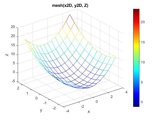
The resulting plot is shown here.
Figure \(\PageIndex{1}\): mesh() 3D plot
.
surf() 3D plot
The surf() function also creates a continous surface 3-dimensional plot. Its usage is the same as the mesh() function.
format short g; format compact; clear all; close all; clc;
%% Create a 3D graph of r^2 = x^2 + y^2 over a grid of points
% 1. Set the x and y axis 1D vectors that define this rectangular grid:
x1D = -3 : 0.5 :3; % 1x13 vector
y1D = -2.5: 0.5 :2.5; % 1x11 vector
%% 2. Matlab's meshgrid() function uses these 1D vectors
% to create 2D arrays of x & y at each point of the rectangular grid.
[x2D, y2D] = meshgrid(x1D,y1D);
%% 3. Compute z(x,y) at each point in the grid.
z = x2D.^2 + 1*x2D + y2D.^2 + 2*y2D;
%% surf(x,y,z) creates a 3D continous surface plot.
figure;
surf(x2D, y2D, z);
title('mesh(x2D, y2D, Z)');
colormap hot % This selects a colormap
colorbar; % This displays the color scale
xlabel('x') % This identifies x-axis
ylabel('y')
zlabel('z')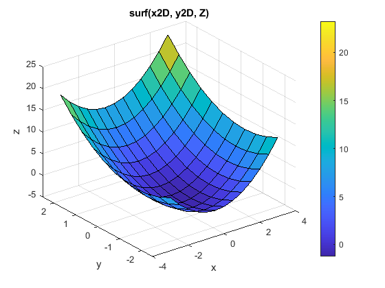
Solution
The resulting plot is shown here.
Figure \(\PageIndex{2}\): surf() 3D plot
See this attached file for images of the colormap options.: colormap_options.pdf
.
contour() Plot
Contour plots are like topographical maps. They display 3D data in a 2D format. The basic syntax is:
contour(x2D, y2D, z);
This can be improved by specifying the contour levels and showing their values:
contour(x2D, y2D, z, levels, 'ShowText','on')); % This creates specified contours and shows their values.
format short g; format compact; clear all; close all; clc;
%% Create a 3D graph of r^2 = x^2 + y^2 over a grid of points
% 1. Set the x and y axis 1D vectors that define this rectangular grid:
x1D = -3 : 0.5 :3; % 1x13 vector
y1D = -2.5: 0.5 :2.5; % 1x11 vector
%% 2. Matlab's meshgrid() function uses these 1D vectors
% to create 2D arrays of x & y at each point of the rectangular grid.
[x2D, y2D] = meshgrid(x1D,y1D);
%% 3. Compute z(x,y) at each point in the grid.
z = x2D.^2 + 1*x2D + y2D.^2 + 2*y2D;
%% contour(x,y,z) creates a continous surface plot.
figure;
levels = [-4: 2: 24]; % Specify the contours
contour(x2D, y2D, z, levels, 'ShowText','on');
title('contour(x2D, y2D, Z), levels, ''ShowText'',''on'')');
colorbar; % This displays the color scale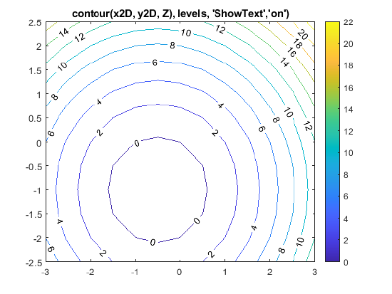
Solution
Resulting plot:
Figure \(\PageIndex{3}\): contour() plot
.
.
colormap Options
|
jet |
 |
|
parula |
 |
|
hsv |
 |
|
hot |
 |
|
cool |
 |
|
spring |
 |
|
summer |
 |
|
autumn |
 |
|
winter |
 |
|
gray |
 |
|
bone |
 |
|
copper |
 |
|
prism |
 |
|
flag |
 |
|
colorcube |
 |
|
lines |
 |