Plate Heat Exchanger

Introduction

Heat exchangers are among the most common equipment in the processing industry. Plate exchangers are compact and versatile. If you have a tour of a local microbrewery, it's highly likely that you'll find plate heat exchangers in use. In terms of engineering fundamentals, our setup allows us to investigate transient heat transfer operations. Specifically, the goals of this project are for you to

• derive the working equations of a batch heating operation,
• apply the results to the operation of a plate heat exchanger,
• apply computer data acquisition, and
• evaluate the overall heat transfer coefficient under different operating conditions.

Background

Because plate heat exchangers are a well-established technology, your key references should be textbooks in heat and mass transfer. In particular,

• Perry's Chemical Engineers' Handbook^[1]is one of the most useful texts for chemical engineers and should be one of the first places you check for any chemical engineering project. A (large) copy is available online.
• Heat Transfer in Process Engineering^[2] is a good, practical text with a chapter specifically on plate heat exchangers. Our library has an electronic copy of this book available through UC-eLinks.
• Unit Operations of Chemical Engineering^[3] provides a useful, empirical correlation (and a worked example!) between common dimensionless numbers (Nu, Re, and Pr) which can be verified experimentally. Our library has several copies of this text and most of the professors should have a copy as well.

Theory

Steady State Operation

<figure class="article-thumb tright show-info-icon" style="width: 309px">

<figcaption>

Figure 1. Heat exchanger details. (a) Temperatures and flow rates for cross-flow plate heat exchanger operating in continuous mode. (b) Temperature change schematic as a function of heat transfer within the heat exchanger. The choice of $\Delta T$ and $q_T$ are arbitrary.

</figcaption> </figure>

A schematic of cross-flow in a plate heat exchanger is provided in Figure 1(a) where $T$ denotes stream temperature, $\omega$ is the stream mass flow rate, and subscripts $c$ and $h$ refer to cold and hot streams. The temperature change of each stream is sketched in Figure 1(b) as a function of total heat $q_T$ transferred from the hot stream to the cold stream. At any point within the exchanger the differential heat $dq$ transferred from hot to cold is

$$dq = U\left(T_h - T_c\right) dA,$$

where $U$ is the overall heat transfer coefficient and $dA$ is the differential area available for heat transfer. As implied by Figure 1(b), the temperature difference $\Delta T = T_h - T_c$ is approximately linear such that

$$\frac{d\left(\Delta T\right)}{dq} = \frac{\Delta T_1 - \Delta T_2}{q_T}.$$

Combining Eqs. (1) and (2) and integrating over the area $A$ of the exchanger we see that

$$q_T = UA\frac{\Delta T_1 - \Delta T_2}{\ln \frac{\Delta T_1}{\Delta T_2}} = UA \Delta T_{lmtd},$$

where $\Delta T_{lmtd}$ is the log-mean temperature difference. Since the assignment of $\Delta T$ was arbitrary, $\Delta T_{lmtd}$ may be made positive in any application simply by reversing the selection of $\Delta T_1$ and $\Delta T_2$.

The total heat $q_T$ transferred from the hot stream to the cold stream can also be determined from the temperature change of either stream by using the general relationship

$$q_T = \omega_c C_{P,c} \left(T_c^{out} - T_c^{in}\right) = \omega_h C_{p,h} \left(T_h^{out} - T_h^{in}\right),$$

where $C_p$ is the heat capacity of the noted stream, and under most circumstances we can approximate $C_{p,c} = C_{p,h} = C_p$. Equating Eqs. (3) and (4) provides two methods to determine $U$ at steady state: $U_c$ based on the cold stream and $U_h$ based on the hot stream. Ideally $U_c = U_h$ because $q_c = q_h = q_T$ but a careful evaluation of $q_T$ via Eq. (4) may reveal more interesting behavior.

As noted above, empirical correlations exist for plate heat exchanger performance.^[4] The general form is

$$\textrm{Nu} = a \textrm{Re}^b \textrm{Pr}^c,$$

where $\textrm{Nu, Re,}$ and $\textrm{Pr}$ are the Nusselt, Reynolds, and Prandtl numbers, and $a, b,$ and $c$ are experimentally determined coefficients. Typically, $b \approx 2/3$ and $c \approx 1/3$ but different authors report different values.^[5] Note that correlations of this form predict different scaling behavior compared to Eqs. (3) and (4).

Batch Operation

<figure class="article-thumb tnone show-info-icon" style="width: 200px">

<figcaption>

Figure 2. Heat exchanger operation under batch conditions for the cold stream. We assume $T_h^{in}$ is approximately constant due to the hot water heater (not shown).

</figcaption> </figure>

For this lab, we simulate batch operation through a cold water loop as shown in Figure 2 wherein a mass $m$ of cold water is drawn from and returned to a common reservoir. The hot water inlet temperature $T_h^{in}$ is assumed to be constant due to the hot water heater (not shown) which continuously heats a hot water reservoir. Assuming constant heat capacity $C_p$ everywhere and a well-mixed reservoir such that $T_m = T_c^{in}$, a control volume around the cold water reservoir implies

$$m C_p \frac{dT_c^{in}}{dt} = \omega_c C_p \left(T_c^{out}- T_c^{in}\right) = UA\Delta T_{lmtd},$$

and we seek various forms to the solution of this equation for the cases of unequal flow ($\omega_c \neq \omega_h$) and equal flow ($\omega_c = \omega_h$). Note that Eq. (6) can be rearranged to give an expression for the cold outlet temperature as,

$$T_c^{out} = T_c^{in} + \frac{m}{\omega_c}\frac{dT_c^{in}}{dt},$$

and the analogous form based on the hot stream gives

$$T_h^{out} = T_h^{in} - \frac{m}{\omega_h}\frac{dT_c^{in}}{dt},$$

which will be useful in the following derivations.

Unequal Flow

Substituting Eqs. (8) and (9) into the definition of $\Delta T_{lmtd}$ gives

$$\Delta T_{lmtd} = \frac{m \left(\frac{1}{\omega_c} - \frac{1}{\omega_h}\right) \frac{dT_c^{in}}{dt}}{\ln\left| \frac{T_h^{in} - T_c^{in} - \frac{m}{\omega_h}\frac{dT_c^{in}}{dt}}{T_h^{in} - T_c^{in} - \frac{m}{\omega_c} \frac{dT_c^{in}}{dt}} \right|}.$$

Thus Eq. (6) becomes

$$\ln\left| \frac{T_h^{in} - T_c^{in} - \frac{m}{\omega_h}\frac{dT_c^{in}}{dt}}{T_h^{in} - T_c^{in} - \frac{m}{\omega_c} \frac{dT_c^{in}}{dt}} \right| = \frac{UA}{C_p}\left(\frac{1}{\omega_c}-\frac{1}{\omega_h}\right).$$

In an effort to simplify the subsequent steps, we'll define

$$\ln K = \frac{UA}{C_p}\left(\frac{1}{\omega_c} - \frac{1}{\omega_h}\right)$$

and

$$T^{\prime} = T_h^{in} - T_c^{in}$$

such that

$$\frac{dT^{\prime}}{dt} = -\frac{dT_c^{in}}{dt}.$$

Now Eq. (10) becomes a separable, first-order, ordinary differential equation of the form

$$\frac{dT^{\prime}}{T^{\prime}} = \frac{1-K}{m\left(\frac{K}{\omega_c}-\frac{1}{\omega_h}\right)}dt.$$

With the initial condition $T_c^{in}\left(t=0\right)=T_c^{in}\left(0\right)$, integration of Eq. (14) gives

$$-\ln \left| \frac{T_h^{in}-T_c^{in}\left(t\right)}{T_h^{in}-T_c^{in}\left(0\right)}\right| =\left[ \frac{\left(K-1\right)\omega_c\omega_h}{m\left(K\omega_h-\omega_c\right )}\right]t,$$

which has the form $f\left(T,t\right) = bt$ and therefore linear regression tools can be used to evaluate $b$ and, by extension, $U$.

Equal Flow

When $\omega_h = \omega_c$, the lines of Figure 1 are parallel by Eq. (4) and hence $\Delta T_1 = \Delta T_2$. The log-mean temperature difference becomes indeterminate but application of L'Hospital's rule (or careful inspection of Eqs. (1) and (2)) implies $\Delta T_{lmtd} = \Delta T_1 = \Delta T_2$, and Eq. (6) becomes

$$mC_p \frac{dT_c^{in}}{dt} = UA\left(T_h^{out} - T_c^{in}\right),$$

where $\Delta T_1$ was chosen arbitrarily. As you should prove to yourself, combined with Eq. (8) and simplified using Eqs. (12) and (13), we are again left with a separable, first-order, ordinary differential equation of the form

$$-\frac{dT^{\prime}}{T^{\prime}} = \frac{1}{\frac{m C_p}{UA} + \frac{m}{\omega}} dt,$$

which may be integrated with the same initial condition as before to give

$$-\ln \frac{T^{\prime}\left(t\right)}{T^{\prime}\left(0\right)} = \frac{1}{\tau_{th}+\tau_r}t,$$

where $\tau_{th} = mC_p / UA$ represents a thermal timescale which relates the thermal mass $m C_p$ of the tank to the rate $UA$ at which thermal energy is changed, and $\tau_r = m/\omega$ represents a residence timescale which relates the mass $m$ of the tank to the rate $\omega$ at which mass is recycled. As expected, the approach temperature $T^{\prime}$ decays exponentially from its initial value $T^{\prime}\left(0\right)$ to zero, and does so on a timescale $\tau$ equal to $\tau_{th} + \tau_r$ (Figure 3). A clever engineer could use these timescales to estimate how long she should operate a system in batch mode to avoid entering the large $\tau$ regime and thus losing her thermal driving force.

<figure class="article-thumb tnone show-info-icon" style="width: 220px">

<figcaption>

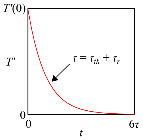
Figure 3. Approach temperature behavior for batch operation with equal flow rates. The red curve is an exponential decay characterized by two timescales as described in the text: $\tau_{th}$, a thermal timescale, and $\tau_r$, a residence timescale.

</figcaption> </figure>

Standard Operating Procedure

Safety

This experiment uses only water and therefore has minimal chemical safety considerations. Nonetheless, relevant chemical information has been listed in Table 1^[6]. In the event of exposure to hot water, run cool water over the affected area and use the emergency protocols at the exits to contact Health and Safety if additional medical attention is required.

Table 1. Chemicals and their formulas, hazards, and suppliers for the plate heat exchanger.

Name^MSDS	Formula	Hazard	Supplier	SKU
Water	H2O		unk	unk

Preparation

1. On the hot water heater, set the red knob to "B" or the desired level. It can take about 30 min before the hot water is available.
2. Open PHE datalogger.vi^[7] on the laptop. Only the first four temperature channels are useful. If errors are reported when the VI is executed, try re-starting the computer and re-booting the DAQ; the latter may be accomplished by unplugging the DAQ, waiting 10 s, then plugging it in again.
3. Familiarize yourself with the piping so that you can identify all streams. Also locate pump power switches, resistance temperature detectors (RTDs, inaccurately referred to as thermocouples), the hot water "buffer" reservoir, and volumetric flow indicators and control valves.
4. Estimate the plate area available for heat transfer and--for batch operation--the mass of water in the cold tank.

Basic Operation

For all operation methods,

• do not run the pumps with zero flow (check the appropriate feed, flow rate, and exit valves),
• do not operate any streams with less than 1 gal/min to avoid cavitation, and
• do not overestimate the quality of the controller on the hot water tank (be ready for variation).

Continuous Operation

1. Set cold-side valves such that one tank is the feed and the other is for discharge.
2. Start data acquisition.
3. Turn on pumps and set flow rates to desired values.
4. Run until steady state is achieved (what does this mean?).
5. Turn off pumps and stop data acquisition.
6. Repeat for desired settings. If necessary, wait for heat to re-heat water.

Batch Operation

1. Move most, but not all, water to a single cold reservoir.
2. Set cold-side valves such that the relevant cold reservoir is both feed and discharge.
3. Repeat steady-state operation procedures 2-5, but stop operation before approach temperature is 10 °C.

Shutdown

1. Turn water heater setting to "Low."
2. Close LabVIEW and shut down the computer.

References

1. ↑ Shilling, R. et al. In: Perry's Chemical Engineers' Handbook, Green, D., Perry, R. Eds., 8th Ed.; McGraw-Hill: New York, 2008; Ch. 11
2. ↑ Cao, E. Heat transfer in process engineering, McGraw-Hill: New York, 2010; Ch. 9.
3. ↑ McCabe, W.; Smith, J.; Harriott, P. Unit Operations of Chemical Engineering, 7th Ed., McGraw-Hill: Boston, 2004; Ch. 15.
4. ↑ McCabe, W.; Smith, J.; Harriott, P. Unit Operations of Chemical Engineering, 7th Ed., McGraw-Hill: Boston, 2004; Ch. 15.
5. ↑ Pradhan, R.; Ravikumar, D.; Pradhan, D. IOSR J. Mech. Civil Eng. 2013, 4, 1-8. You can find a copy of this paper here, and Table 1 is of particular relevance.
6. ↑ Read the indicated MSDS for water and you'll learn lots of interesting things about water, including that water is non-flammable and that water should be mopped up in the event of a spill. SCIENCE!!!
7. ↑ C:\Documents and Settings\CENG176 Laptop\Desktop\PHE\PHE datalogger.vi