8.3.3: Methods of Harnessing Tidal Power
- Page ID
- 85139
According to an Encyclopedia Britannica article, the total power contained in tides worldwide is estimated to be 3000 GW – it’s three times the total electricity generating power installed in the US, and about 20% of the global power consumption. Of those 3000 GW, it is estimated that between 120 and 400 GW can be generated by tidal barrages, and the remainder by underwater turbines capturing power from tidal currents.
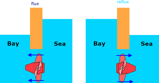
Tidal Barrages. This technology is now well established. The idea is very simple: one needs a “tidal basin” – a relatively narrow bay, a river estuary, or a fjord, and to build a “barrage” – a dam that would capture the high tide water. Then, during the low tide period, this water can be send to turbines. Essentially, it’s the same operating scheme as that used by conventional hydropower plants with dams built on rivers. However, those power plants work only “one-way” – naturally, the high water level is on the “upriver” side of the dam, and water, after flowing through the turbines, continues flowing “downriver”. In contrast, a barrage plant can use a “two-way cycle”, in which the same water flows twice through the turbines. Suppose that the cycle begins when the “tidal basin” – the reservoir behind the barrage is empty, and there is a high-tide water level on the sea-side of the barrage. Then valves (called ”sluice gates”) are set open, letting water to flow in through the turbines, until the reservoir gets filled. Now, the valves are closed, and the power plant has to pause and wait for the low tide. When it happens, the valves are again opened and water from the filled reservoir flows back to the sea, again passing through the turbines, until the reservoir is emptied. The valves are now closed and the plant takes another pause, waiting for the next high tide – when it comes, a new cycle begins. So, during a half-day cycle, there are two generating sessions, each followed by a pause.
In France, the Rance Tidal Power Station built at the mouth of the La Rance river estuary has been operating since 1966. Its location is very favorable because the tidal range in the estuary is as high as 8 meters. The plant’s maximum power is 240 MW (but due to the natural intermittency of tidal the average power is only 57 MW, corresponding to a capacity factor of about 24%. Another slightly larger facility (254 MW)is the Sihwa Lake Tidal Power Station in South Korea, commissioned in 2011.


As of the beginning of the 2018 year, there are no other existing tidal barrage power plants with power comparable to the two listed above. Nonetheless, there are several ongoing projects of building more such facilities at different parts of the world.
One of the reasons for the slow progress in developing new major barrage power plant is certainly the high cost of building large dams. After the construction is completed, the energy is “essentially for free”, the only costs are due to maintenance and service. But in the case of the La Rance plan it took 20 years to pay back the initial investment.
Tidal Stream Turbines. A much less expensive way is to harness the energy of tidal currents, often referred to as tidal streams. No huge construc- tions, no earthmoving, no many thousand tons of reinforced concrete are needed.
The “tidal stream generators”, as they are called, are pretty similar to wind turbines. One can use the same math as that used for wind turbines to calculate the expected power output from a single unit – namely, the Eq. 6.2 from the Windpower chapter, with \( A = \pi R^2 \):
\[ P=\frac{\pi R^{2} \rho V^{3}}{2} \]
where \(R\), as before, is the radius of the turbine, and now \(V\) is the speed not of wind, but of the current, and \(\rho\) is the density not of the air, but now of the salty seawater, approximately \(1025 \mathrm{~kg} / \mathrm{m}^{3}\).
Let's do an example: a turbine of \(10 \mathrm{m}\) diameter \((R=5 \mathrm{~m})\) is placed in the current in Cook Strait. The maximum current speed over there, as we remember, is 4 knots \(=4 \times 1852 \mathrm{~m} /\) hour \(=7408 \mathrm{~m} /\) hour \(=7408 / 3600\) \(\mathrm{m} / \mathrm{s}=2.06 \mathrm{~m} / \mathrm{s}\). So, \(P=1 / 2 \times\left(\pi \times 5^{2} \times 1025 \times 2.06^{3}\right) \mathrm{W}=352 \mathrm{~kW}\). Well, but the Betz Limit does apply, and the efficiency factor, so let's take only one half of this. \(170 \mathrm{~kW}\), it's still a very decent power, it's more than what one hundred average American households consume.
Another interesting problem: let's make a rough estimate \({ }^{1}\), what's the total energy of the water comprising the tidal current in the Cooks Strait? Why only a rough estimate? Well, we don't know all essential parameters, we have to base our calculation on a few "guesses". We know that the maximum current speed in the Strait is \(2.06 \mathrm{~m} / \mathrm{s}\), that is \(20 \mathrm{~km}\) wide, and that its average depth is slightly above 100 fathoms. One fathom is 6 feet. Well, but
we don't know whether the current speed is uniform all the way from the surface to the bottom, or perhaps it isn't? Let's try to make our estimates "conservative", it's always safer to "undershoot" than to "overshoot". So, let's assume that the speed \(V=2.06 \mathrm{~m} / \mathrm{s}\) applies only to the depth of 100 \(\mathrm{m}\). Now, in order to obtain the total energy, we need to take into account the entire water in the strait. And how long it is? Again we have to make a guess: let it be \(20 \mathrm{~km}\). So, in our "model", it's like a river \(20000=20^{4}\) meters wide, \(2 \times 10^{4} \mathrm{~m}\) long, and \(10^{2} \mathrm{~m}\) deep, and all that seawater is flowing with a speed of \(2.06 \mathrm{~m} / \mathrm{s}\). The total volume of the water flowing is:
\[
v=\left(2 \times 10^{4}\right) \times\left(2 \times 10^{4}\right) \times 10^{2} \mathrm{~m}^{3}=4 \times 10^{10} \mathrm{~m}^{3} .
\]
For calculating the total kinetic energy we need not the volume, but the mass of the moving object - so we multiply the volume by the density of seawater, \(1025 \mathrm{~kg} / \mathrm{m}^{3}\), to obtain \(m=4.1 \times 10^{13}\) kilograms. The last step is to use the well-known formula for kinetic energy:
\[
K=m V^{2} / 2=4.1 \times 10^{13} \times 2.06^{2} / 2 \mathrm{~kg} \cdot \mathrm{m}^{2} / \mathrm{s}^{2}=8.7 \times 10^{13} \mathrm{~J}
\]
Would the fact matter that the turbine from the preceding example is "stealing" energy from the tidal flow with a rate of \(170 \mathrm{~kW}=170\) ooo W \(=1.7 \times 10^{5}\) \(\mathrm{J} / \mathrm{s}\) ? Suppose that the "theft" is continued for 3 hours \(10^{4}\) seconds, approximately the time period the high tide lasts. So, the total "stolen" amount is \(1.7 \times 10^{9} \mathrm{~J}\). Is it much? Let's check:
\[
\frac{1.7 \times 10^{9}}{8.7 \times 10^{13}}=1.95 \times 10^{-5}=0.00195 \%
\]
It's only a tiny part of the total energy of the current. It shows that one can install as many as 500 such turbines as we have considered in the first example, and they will extract only about one percent of the total power of the tidal current. It does not seem likely that the natural flow of tide water in the Cook Strait would be significantly affected by such turbine system.

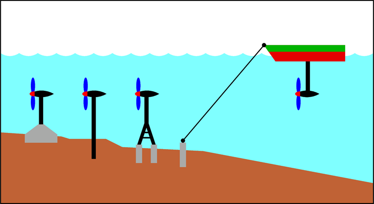
One more interesting fact about tidal stream turbines. Installing them on the waterway bottom in a similar way as installing wind turbines on dry land – it is, at the top of a tower erected from a solid foundation – is not the only option. There is even a simpler way: to use a flat bottom of a barge as the base of a “pointing down tower”, and mount the turbine at the lower end of such “tower”. The barge should be moored, of course, to sturdy posts at the bottom (or, if the tidal stream flows in a narrow canal, to rocks on both sides of such passage).
Harnessing power of tidal streams has several advantages. The machinery is relatively simple. There is no need to permanently change the landscape, because all components of the system may be either hidden underwater, or – if a floating system is used – a moored barge is never thought of as a permanent object distorting the landscape. In contrast to wind turbines that may kill birds, the rotation speed of underwater turbines is much slower, so they may not pose a serious threat to aquatic life (but there, nevertheless, some other concerns related to the ecosystems).
______________________________________________________
1. By an estimate, a physicist usually means a result that differs no more than an order of magnitude from the actual value. And an order of magnitude means: ten times larger, or ten times smaller.

