4.1: Buoyancy force distribution on ships

Last updated
Save as PDF

Page ID: 95300

$ \newcommand{\vecs}[1]{\overset { \scriptstyle \rightharpoonup} {\mathbf{#1}} } $

$ \newcommand{\vecd}[1]{\overset{-\!-\!\rightharpoonup}{\vphantom{a}\smash {#1}}} $

$ \newcommand{\id}{\mathrm{id}}$ $ \newcommand{\Span}{\mathrm{span}}$

( \newcommand{\kernel}{\mathrm{null}\,}\) $ \newcommand{\range}{\mathrm{range}\,}$

$ \newcommand{\RealPart}{\mathrm{Re}}$ $ \newcommand{\ImaginaryPart}{\mathrm{Im}}$

$ \newcommand{\Argument}{\mathrm{Arg}}$ $ \newcommand{\norm}[1]{\| #1 \|}$

$ \newcommand{\inner}[2]{\langle #1, #2 \rangle}$

$ \newcommand{\Span}{\mathrm{span}}$

$ \newcommand{\id}{\mathrm{id}}$

$ \newcommand{\Span}{\mathrm{span}}$

$ \newcommand{\kernel}{\mathrm{null}\,}$

$ \newcommand{\range}{\mathrm{range}\,}$

$ \newcommand{\RealPart}{\mathrm{Re}}$

$ \newcommand{\ImaginaryPart}{\mathrm{Im}}$

$ \newcommand{\Argument}{\mathrm{Arg}}$

$ \newcommand{\norm}[1]{\| #1 \|}$

$ \newcommand{\inner}[2]{\langle #1, #2 \rangle}$

$ \newcommand{\Span}{\mathrm{span}}$ $ \newcommand{\AA}{\unicode[.8,0]{x212B}}$

$ \newcommand{\vectorA}[1]{\vec{#1}} % arrow$

$ \newcommand{\vectorAt}[1]{\vec{\text{#1}}} % arrow$

$ \newcommand{\vectorB}[1]{\overset { \scriptstyle \rightharpoonup} {\mathbf{#1}} } $

$ \newcommand{\vectorC}[1]{\textbf{#1}} $

$ \newcommand{\vectorD}[1]{\overrightarrow{#1}} $

$ \newcommand{\vectorDt}[1]{\overrightarrow{\text{#1}}} $

$ \newcommand{\vectE}[1]{\overset{-\!-\!\rightharpoonup}{\vphantom{a}\smash{\mathbf {#1}}}} $

$ \newcommand{\vecs}[1]{\overset { \scriptstyle \rightharpoonup} {\mathbf{#1}} } $

$ \newcommand{\vecd}[1]{\overset{-\!-\!\rightharpoonup}{\vphantom{a}\smash {#1}}} $

4.3.2 Buoyancy force distribution on ships

The simple uniform buoyancy distribution acting on the barge in example 4.2 is an exception to the buoyancy distributions found in practice. It is true that equilibrium requires the total buoyant upthrust to equal the weight of the ship and its contents. However, the distribution of the buoyancy and weight along the length of the ship is not necessarily the same. The difference in the magnitudes of the buoyancy and weight distribution intensities is the applied load intensity f_y(z). In ship design three conditions are recognized to compute f_y(z) for the same ship. These conditions are called

the still water condition,
the sagging condition, and
the hogging condition.

A more detailed account of these conditions on the longitudinal bending of the ship is given by Muckle (1967) and Zubaly (1996), and here we only summarize the basic ideas.

A ship in still water is shown in figure 4.12, and a section A-A between z and $z + dz$ $math-516.png$ is also shown. Archimedes’s principle asserts that the buoyant upthrust is equal to the weight of the fluid displaced. Let A(z) denote the submerged cross section at z, and let γ denote the specific weight (force per volume) of the fluid. The differential buoyancy force dF_b acting on the ship over a differential length dz is

The hull of a ship is shown, with z beginning with 0 at the stern, and growing as it moves towards the bow. It is initially only above the waterline, before having portions both above and below, with approximately two thirds of the hull below water. A cross-section cap A dash cap A is marked at two-thirds of the length facing the stern. Cross section cap A cap A is shown with area cap A of z times dz. A bouyant force d cap F sub b is applied at the center of the barge’s bottom. 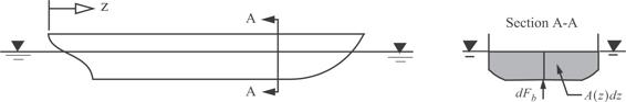— Fig. 4.12 A ship in still water.

$\begin{align} d F_{b} = γ A (z) d z . & (4.32) \end{align}$ $math-517.png$

Consequently, the buoyant upthrust per unit ship length, which we designate f_b, is equal to $γ A (z)$ $math-518.png$ ; i.e.,

$\begin{align} f_{b} = \frac{d F_{b}}{d z} = γ A (z) . & (4.33) \end{align}$ $math-519.png$

A curve of f_b for a ship as well as the weight per unit length is shown in figure 4.13. Overall equilibrium requires the area under these curves to have the same magnitude. If the submerged cross section is uniform in z, as is the case for the barge in example 4.2, the distribution of the buoyancy per unit length f_b is a constant.

The plot of weight per length of the ship is shown to grow to a small value that slowly increases before drastically increasing to much larger values between one fourth and three fourths of the length, before then dropping back to smaller values that decrease linearly back to zero. The buoyancy per length plot is much smoother than the weight per length plot, growing to values just below those of the larger inner values of the weight per length plot before decreasing back to zero at the ends. — Fig. 4.13 Conceptual longitudinal weight and buoyancy distributions acting on a ship.

At sea a ship is subject to waves, and this alters the buoyancy distribution. For longitudinal bending of the ship two extreme static conditions are assumed: sagging and hogging. In each condition, the length of the wave is assumed to be the length of the ship. This is an “accepted” assumption for the worst buoyancy distribution causing the most severe bending of the ship.

The sagging condition is shown in figure 4.14(a). The wave crests are at the bow and stern, and the wave trough is amidships. A schematic of the buoyancy per unit length is shown below the ship in figure 4.14(a). The immersed cross section is the largest at or near the wave crests, and is least near the trough. The intensity of the buoyancy distribution reflects this. In this condition the deck sags and is in compression while the bottom is in tension. The worst location to concentrate the cargo in the ship is amidships, as this will result in the largest bending moment.

A ship hull is shown with the water higher at the bow and stern than in the center, resulting in a concentrated weight at the center. The resulting distributed load f sub b thus has peaks that mirror the water level, starting from zero on each end and having peaks near the edges, while the center sags. A ship hull is shown with the water higher at the center of the ship, resulting in weight concentrations near the bow and stern. The distributed load f sub b mirrors the water distribution, beginning from zero before rising to a maximum in the center and falling to zero at the other edge, similar to a bell curve. 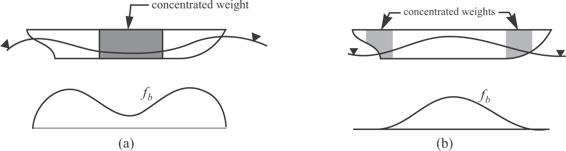— Fig. 4.14 Longitudinal bending conditions for a ship. (a) Sagging. (b) Hogging.

The hogging condition is depicted in figure 4.14(b). Here the wave troughs are at bow and stern, and the crest is amidships. The immersed cross section is greatest near amidships and is least near bow and stern. The distribution of the buoyancy per unit length f_b, shown in figure 4.14(b), reflects this situation. In hogging the deck is in tension and the bottom is in compression. The worst possible locations to concentrate cargo is fore and aft, as this will produce the greatest bending moment in the ship.

4.3.3 Properties of plane areas

First and second area moments of the cross-sectional area need to be determined before evaluating eq. (4.6) for the normal stress. Analytical procedures were used in Example 3.1 on page 44 to compute first and second area moments for a thin-walled bar. Frequently, the composite area technique in conjunction with the parallel axis theorem are used to determine these geometric properties.

A global cap X cap Y axis system is centered at point cap O. A cross sectional area is shown centered at centroid cap C, resembling a capital Z with a straight center section, rather than slanted. The cross section is of thickness t of s, with s beginning from the bottom right corner and moving through the structure towards the top left corner. Centroid cap C is located at cap X sub c and cap Y sub c, with a local x y axis system centered at cap C and parallel to the global cap X cap Y axis system. 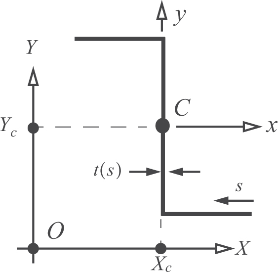— Fig. 4.15 Parallel Cartesian axes systems.

Parallel axis theorem. Consider two parallel axes systems in the cross section. The origin of the Cartesian axes x and y coincide with the centroid of the cross-sectional area, which is labeled C in figure 4.15. The second Cartesian system X and Y has its origin at an arbitrary point O, the X-axis is parallel to the x-axis, and the Y -axis is parallel to the y-axis. The location of the centroid in the X and X system is denoted by coordinate values (X_c, Y_c). Usually the X and Y system is selected as something convenient to start with, and the first and second area moments with respect to the X and Y system are computed or looked up in tables. Then the (X_c, Y_c) coordinates of the centroid are computed and the parallel axis theorem is used to find the second area moments in the x and y system.

For a thin-walled bar the area element is dA = t(s)ds, in which s denotes the arc-length along the contour c, and t(s) denotes the thickness of the wall. In general, the thickness may vary smoothly with arc-length, but its magnitude must remain small with respect to the overall dimensions of the cross section. An abrupt change in thickness is modeled by a step change in thickness at a junction. The area of the cross section is given by

$\begin{align} A = \int_{c} t (s) d s . & (4.34) \end{align}$ $math-520.png$

In the X and Y system, the first area moments are defined as

$\begin{align} Q_{X} = \int_{c} Y t d s Q_{Y} = \int_{c} X t d s . & (4.35) \end{align}$ $math-521.png$

The relationship between the two parallel coordinate systems is determined from the location of a generic point s on the contour in each system. This relationship is

$\begin{align} X (s) = X_{C} + x (s) Y (s) = Y_{C} + y (s) . & (4.36) \end{align}$ $math-522.png$

If eq. (4.36) is substituted into eq. (4.35), we get

$\begin{align} Q_{X} = Y_{C} A + Q_{x} Q_{Y} = X_{C} A + Q_{y} . & (4.37) \end{align}$ $math-523.png$

where

$\begin{align} Q_{x} = \int_{c} y (s) t (s) d s Q_{y} = \int_{c} x (s) t (s) d s . & (4.38) \end{align}$ $math-524.png$

Since the origin of the x and y system is at the centroid, the first moments Q_x and Q_y are zero by definition. Setting Q_x = 0 and Q_y = 0 in eq. (4.37), we can solve to find the location of the centroid as

$\begin{align} X_{C} = \frac{Q_{Y}}{A} Y_{C} = \frac{Q_{X}}{A} . & (4.39) \end{align}$ $math-525.png$

In the X and Y coordinate system the second area moments are defined by

$\begin{align} I_{X X} = \int_{c} Y^{2} t d s I_{Y Y} = \int_{c} X^{2} t d s I_{X Y} = \int_{c} X Y t d s . & (4.40) \end{align}$ $math-526.png$

Second area moments are often called moments of inertia in analogy to moments of inertia of mass elements used in rigid body dynamics. The fact that eq. (4.40) is second moments of area elements and not mass elements should be kept in mind even if the terminology “moments of inertia” is used in the context of beam bending. Now substitute eq. (4.36) for the X and Y coordinates into eq. (4.40) to get

$\begin{align} I_{X X} = Y_{C}^{2} A + 2 Y_{C} Q_{x} + I_{x x} I_{Y Y} = X_{C}^{2} A + 2 X_{C} Q_{y} + I_{y y} I_{X Y} = X_{C} Y_{C} A + X_{C} Q_{x} + Y_{C} Q_{y} + I_{x y}, & (4.41) \end{align}$ $math-527.png$

where the second area moments with respect to the centroid are given by

$\begin{align} I_{x x} = \int_{c} y^{2} t d s I_{y y} = \int_{c} x^{2} t d s I_{x y} = \int_{c} x y t d s . & (4.42) \end{align}$ $math-528.png$

Since the origin of the x and y coordinates is at the centroid $Q_{x} = Q_{y} = 0$ , and eq. (4.41) reduces to

$\begin{align} I_{X X} = Y_{C}^{2} A + I_{x x} I_{Y Y} = X_{C}^{2} A + I_{y y} I_{X Y} = X_{C} Y_{C} A + I_{x y} . & (4.43) \end{align}$ $math-530.png$

Equation (4.41) is the generalized parallel axis theorem, but in problem solving we usually use eq. (4.39) to locate the centroid and then the parallel axis theorem reduces to the use of eq. (4.43). Note that eq. (4.42) shows that I_xx and I_yy for real areas are always positive in value with dimensional units of L⁴. The product area moment I_xy can be positive, zero, or negative in value. The product area moment I_xy is zero if either the x-axis or y-axis is an axis of symmetry of the cross section.

Radii of gyration. Define radii of gyration by

$\begin{align} r_{x x} = \sqrt{I_{x x} / A} r_{y y} = \sqrt{I_{y y} / A} . & (4.44) \end{align}$ $math-531.png$

The radii of gyration (4.44) have dimensional units of length. However, the radii of gyration do not locate a physically significant point in the cross section. For example, r_XX ≠ Y_c + r_xx, where r_XX it the radius of gyration with respect to the X-axis. (Using the parallel axis theorem, the relation between the radius of gyration about the X-axis to the x-axis is $r_{X X}^{2} = Y_{C}^{2} + r_{x x}^{2}$ $math-532.png$ .)

Composite area technique. The composite area technique for computing the centroid and second area moments is a method applicable to cross-sectional areas that can be subdivided into simple geometric shapes whose properties are known. An entire area A is subdivided into N sub-areas A_i, $i = 1, 2, \dots, N$ $math-533.png$ as shown in figure 4.16(a). Known properties of the i-th sub-area are its centroid denoted by C_i, and $A_{i}, {(I_{x x})}_{i}, {(I_{y y})}_{i}, {(I_{x y})}_{i}$ $math-534.png$ . Sub-area coordinate axes are denoted by (x_i, y_t) with origin at C_i. Reference axes are denoted by (X, Y) with origin at point O. The x_i-axis is parallel to the X-axis, and the y_i-axis is parallel to the Y -axis. Coordinates (X_i, Y_i) in the reference system locate the centroid C_i of the i-th sub-area.

An area cap A within the global cap X cap Y plane centered at origin cap O. It is divided into cap N sub-sections of arbitrary shape. Each i-th sub section has a local centroid cap C sub i located at cap X sub i and cap Y sub i, and local axes x sub i and y sub i parallel to the global system and centered at cap C sub i. For the total area cap A, the global centroid cap C is located at cap X sub cap C and cap Y sub cap C, with local x and y axes parallel to the global system. 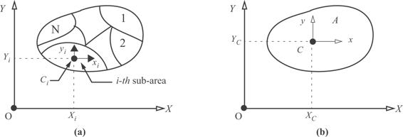— Fig. 4.16 (a) Division of area A into sub-areas. (b) Assembled properties of area A.

The pertinent equations for the assembled area properties are

$\begin{align} A = \sum_{i = 1, 2, \dots}^{N} A_{i} A Y_{C} & = \sum_{i = 1, 2, \dots}^{N} Y_{i} A_{i} A X_{c} = \sum_{i = 1, 2, \dots}^{N} X_{i} A_{i}, and & (4.45) \\ I_{X X} = \sum_{i = 1, 2, \dots}^{N} {(I_{x x} + Y^{2} A)}_{i} I_{Y Y} & = \sum_{i = 1, 2, \dots}^{N} {(I_{y y} + X^{2} A)}_{i} I_{X Y} = \sum_{i = 1, 2, \dots}^{N} {(I_{x y} + X Y A)}_{i} . & (4.46) \end{align}$ $math-535.png$

The coordinates (X_C, Y_C) of the centroid C for the entire area shown in figure 4.16(b) are computed from the last two expressions in eq. (4.45). The origin of the parallel coordinate system x-y is located at the centroid C as shown in figure 4.16(b). The parallel axis theorem (4.43) is used to find the second area moments about centroidal system x-y after the second area moments in the reference system are determined from eq. (4.46).

For branches that can be represented by a thin-walled rectangular area, we can obtain simple formulas for the second area moments. Consider a thin rectangular area, where $0 < t ≪ b$ $math-536.png$ . The contour is a straight line inclined at a angle θ as is shown in figure 4.17. The contour coordinate is denoted by s, and the area element is dA = tds. The x and y coordinates of the point s on the contour are given by $x = s cos ϕ$ $math-537.png$ and $y = s sin ϕ$ $math-538.png$ .

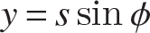Hence, the second area moments are computed from

$\begin{align} I_{x x} & = \int_{- b / 2}^{b / 2} {(s sin θ)}^{2} t d s = \frac{b^{3} t}{12} {sin}^{2} θ \\ I_{y y} & = \int_{- b / 2}^{b / 2} {(s cos θ)}^{2} t d s = \frac{b^{3} t}{12} {cos}^{2} θ . & (4.47) \\ I_{x y} & = \int_{- b / 2}^{b / 2} (s sin θ) (s cos θ) t d s = \frac{b^{3} t}{12} sin θ cos θ \end{align}$ $math-539.png$

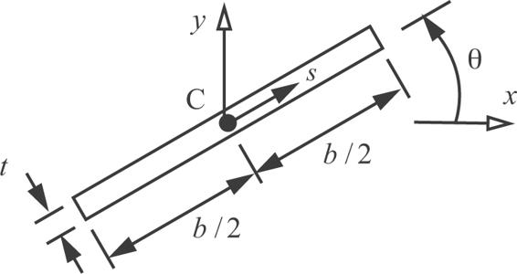
A rectangular area of length b and thickness t is shown. The area’s centroid, cap C, is located at b over 2 from each end, and is the center of the local x y axis system. The area is rotated by angle theta counterclockwise from the local x axis, with lengthwise distance s defined as 0 at cap C, positive up and to the right, and negative down and to the left. — Fig. 4.17 Thin rectangular area inclined at an angle θ.

Example 4.3 Thin-walled zee section properties by the composite area technique

Determine the centroid and the second area moments for the thin-walled zee section shown in figure 4.18. The section is subdivided into three rectangular branches. One branch corresponds to the web and two branches correspond to the flanges.

The cross section resembling a straightened cap Z is divided into three subsections. Section 1 is the bottom horizontal section of length b, with a local centroid located b over 2 along the cap X axis from cap O and cap Y of 0. Section 2 is the vertical section of length 2 b, with a local centroid located b above cap O along the cap Y axis and cap X of 0. Section 3 is the top horizontal section of length b, with a local centroid located negative b over 2 along the cap X axis from cap O and 2 b above cap O on the cap Y axis. All three segments have local x sub i and y sub i axes parallel to the cap X and cap Y axes, with i corresponding to segment. The same figure as before is now simplified to have a single set of local x and y axes centered at centroid cap C, located cap Y sub cap C above cap O. All 3 sections have thickness t. 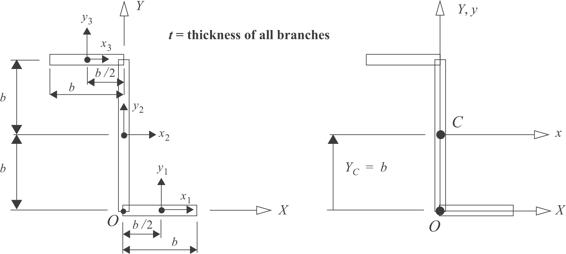— Fig. 4.18 Zee section approximated by three rectangular branches.

Solution. First we find the centroid. Equation (4.45) is represented in table 4.1 shown below.

Summation of the appropriate columns gives

$\begin{align} A = 4 b t X_{c} A = 0 Y_{c} A = 4 b^{2} t, & (a) \end{align}$ $math-540.png$

so that the centroid has coordinates X_c = 0 and Y_c = b.

Table 4.1 Areas and first area moments for the zee section

i	A_i	X_i	Y_i	X_iA_i	Y_iA_ii
1	bt	b/2	0	b²t∕2	0
2	2bt	0	b	0	2b²t
3	bt	−b/2	2b	−b²t/2	2b²t
Sum	4bt			0	4b²t

The second area moments are computed for the reference coordinate system (X, Y) using table 4.2 shown below. Note that for the local coordinate systems originating at the centroid in each branch we can identify the angle θ in eq. (4.47) as θ₁ = 0^°, θ₂ = 90^°, and θ₃ = 0^°. These values of the angle θ in each branch are used to compute the local second area moments in each rectangular branch via eq. (4.47).

Table 4.2 Second area moments for each branch of the zee section

i	$Y_{i}^{2} A_{i}$ $math-541.png$	$(I_{x x})_{i}$ $math-542.png$	$X_{i}^{2} A_{i}$ $math-543.png$	$(I_{y y})_{i}$ $math-544.png$	X_iY_iA_i
1	0	0	b³t/4	b³t∕12	0
2	(b²)2bt	(2b)³t∕12	0	0	0
3	(2b)²bt	0	b³t∕4	b³t∕12	− b³t
Sum	6b³t	2b³t∕3	b³t∕2	b³t∕6	− b³t

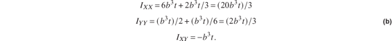
From the summation of the columns, the second area moments in the (X, Y) system via eq. (4.46) are

$\begin{gathered} I_{X X} = 6 b^{3} t + 2 b^{3} t / 3 = (20 b^{3} t) / 3 \\ I_{Y Y} = (b^{3} t) / 2 + (b^{3} t) / 6 = (2 b^{3} t) / 3 \\ I_{X Y} = - b^{3} t . \end{gathered} (b)$ $math-546.png$

Now we use the parallel axis theorem to transfer these moments to the x-y system. Equation (4.43) gives

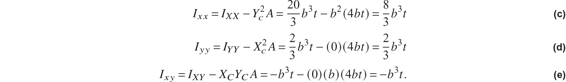
$\begin{align} I_{x x} = I_{X X} - Y_{c}^{2} A = \frac{20}{3} b^{3} t - b^{2} (4 b t) = \frac{8}{3} b^{3} t & (c) \\ I_{y y} = I_{Y Y} - X_{c}^{2} A = \frac{2}{3} b^{3} t - (0) (4 b t) = \frac{2}{3} b^{3} t & (d) \\ I_{x y} = I_{X Y} - X_{C} Y_{C} A = - b^{3} t - (0) (b) (4 b t) = - b^{3} t . & (e) \end{align}$ $math-547.png$

■

Search

Text Color

Text Size

Margin Size

Font Type

4.3.2 Buoyancy force distribution on ships

4.3.3 Properties of plane areas