Home
Under Construction
Aerospace Structures (Johnson)
6: Applications of Castigliano’s Theorems
6.3: Castigliano’s second theorem and statically indeterminate structures

6.3: Castigliano’s second theorem and statically indeterminate structures

Last updated
Save as PDF

Page ID: 95307

$ \newcommand{\vecs}[1]{\overset { \scriptstyle \rightharpoonup} {\mathbf{#1}} } $

$ \newcommand{\vecd}[1]{\overset{-\!-\!\rightharpoonup}{\vphantom{a}\smash {#1}}} $

$ \newcommand{\id}{\mathrm{id}}$ $ \newcommand{\Span}{\mathrm{span}}$

( \newcommand{\kernel}{\mathrm{null}\,}\) $ \newcommand{\range}{\mathrm{range}\,}$

$ \newcommand{\RealPart}{\mathrm{Re}}$ $ \newcommand{\ImaginaryPart}{\mathrm{Im}}$

$ \newcommand{\Argument}{\mathrm{Arg}}$ $ \newcommand{\norm}[1]{\| #1 \|}$

$ \newcommand{\inner}[2]{\langle #1, #2 \rangle}$

$ \newcommand{\Span}{\mathrm{span}}$

$ \newcommand{\id}{\mathrm{id}}$

$ \newcommand{\Span}{\mathrm{span}}$

$ \newcommand{\kernel}{\mathrm{null}\,}$

$ \newcommand{\range}{\mathrm{range}\,}$

$ \newcommand{\RealPart}{\mathrm{Re}}$

$ \newcommand{\ImaginaryPart}{\mathrm{Im}}$

$ \newcommand{\Argument}{\mathrm{Arg}}$

$ \newcommand{\norm}[1]{\| #1 \|}$

$ \newcommand{\inner}[2]{\langle #1, #2 \rangle}$

$ \newcommand{\Span}{\mathrm{span}}$ $ \newcommand{\AA}{\unicode[.8,0]{x212B}}$

$ \newcommand{\vectorA}[1]{\vec{#1}} % arrow$

$ \newcommand{\vectorAt}[1]{\vec{\text{#1}}} % arrow$

$ \newcommand{\vectorB}[1]{\overset { \scriptstyle \rightharpoonup} {\mathbf{#1}} } $

$ \newcommand{\vectorC}[1]{\textbf{#1}} $

$ \newcommand{\vectorD}[1]{\overrightarrow{#1}} $

$ \newcommand{\vectorDt}[1]{\overrightarrow{\text{#1}}} $

$ \newcommand{\vectE}[1]{\overset{-\!-\!\rightharpoonup}{\vphantom{a}\smash{\mathbf {#1}}}} $

$ \newcommand{\vecs}[1]{\overset { \scriptstyle \rightharpoonup} {\mathbf{#1}} } $

$ \newcommand{\vecd}[1]{\overset{-\!-\!\rightharpoonup}{\vphantom{a}\smash {#1}}} $

$\newcommand{\avec}{\mathbf a}$ $\newcommand{\bvec}{\mathbf b}$ $\newcommand{\cvec}{\mathbf c}$ $\newcommand{\dvec}{\mathbf d}$ $\newcommand{\dtil}{\widetilde{\mathbf d}}$ $\newcommand{\evec}{\mathbf e}$ $\newcommand{\fvec}{\mathbf f}$ $\newcommand{\nvec}{\mathbf n}$ $\newcommand{\pvec}{\mathbf p}$ $\newcommand{\qvec}{\mathbf q}$ $\newcommand{\svec}{\mathbf s}$ $\newcommand{\tvec}{\mathbf t}$ $\newcommand{\uvec}{\mathbf u}$ $\newcommand{\vvec}{\mathbf v}$ $\newcommand{\wvec}{\mathbf w}$ $\newcommand{\xvec}{\mathbf x}$ $\newcommand{\yvec}{\mathbf y}$ $\newcommand{\zvec}{\mathbf z}$ $\newcommand{\rvec}{\mathbf r}$ $\newcommand{\mvec}{\mathbf m}$ $\newcommand{\zerovec}{\mathbf 0}$ $\newcommand{\onevec}{\mathbf 1}$ $\newcommand{\real}{\mathbb R}$ $\newcommand{\twovec}[2]{\left[\begin{array}{r}#1 \\ #2 \end{array}\right]}$ $\newcommand{\ctwovec}[2]{\left[\begin{array}{c}#1 \\ #2 \end{array}\right]}$ $\newcommand{\threevec}[3]{\left[\begin{array}{r}#1 \\ #2 \\ #3 \end{array}\right]}$ $\newcommand{\cthreevec}[3]{\left[\begin{array}{c}#1 \\ #2 \\ #3 \end{array}\right]}$ $\newcommand{\fourvec}[4]{\left[\begin{array}{r}#1 \\ #2 \\ #3 \\ #4 \end{array}\right]}$ $\newcommand{\cfourvec}[4]{\left[\begin{array}{c}#1 \\ #2 \\ #3 \\ #4 \end{array}\right]}$ $\newcommand{\fivevec}[5]{\left[\begin{array}{r}#1 \\ #2 \\ #3 \\ #4 \\ #5 \\ \end{array}\right]}$ $\newcommand{\cfivevec}[5]{\left[\begin{array}{c}#1 \\ #2 \\ #3 \\ #4 \\ #5 \\ \end{array}\right]}$ $\newcommand{\mattwo}[4]{\left[\begin{array}{rr}#1 \amp #2 \\ #3 \amp #4 \\ \end{array}\right]}$ $\newcommand{\laspan}[1]{\text{Span}\{#1\}}$ $\newcommand{\bcal}{\cal B}$ $\newcommand{\ccal}{\cal C}$ $\newcommand{\scal}{\cal S}$ $\newcommand{\wcal}{\cal W}$ $\newcommand{\ecal}{\cal E}$ $\newcommand{\coords}[2]{\left\{#1\right\}_{#2}}$ $\newcommand{\gray}[1]{\color{gray}{#1}}$ $\newcommand{\lgray}[1]{\color{lightgray}{#1}}$ $\newcommand{\rank}{\operatorname{rank}}$ $\newcommand{\row}{\text{Row}}$ $\newcommand{\col}{\text{Col}}$ $\renewcommand{\row}{\text{Row}}$ $\newcommand{\nul}{\text{Nul}}$ $\newcommand{\var}{\text{Var}}$ $\newcommand{\corr}{\text{corr}}$ $\newcommand{\len}[1]{\left|#1\right|}$ $\newcommand{\bbar}{\overline{\bvec}}$ $\newcommand{\bhat}{\widehat{\bvec}}$ $\newcommand{\bperp}{\bvec^\perp}$ $\newcommand{\xhat}{\widehat{\xvec}}$ $\newcommand{\vhat}{\widehat{\vvec}}$ $\newcommand{\uhat}{\widehat{\uvec}}$ $\newcommand{\what}{\widehat{\wvec}}$ $\newcommand{\Sighat}{\widehat{\Sigma}}$ $\newcommand{\lt}{<}$ $\newcommand{\gt}{>}$ $\newcommand{\amp}{&}$ $\definecolor{fillinmathshade}{gray}{0.9}$

6.4 Castigliano’s second theorem and statically indeterminate structures

A statically indeterminate structure is one in which the number of unknown forces exceeds the number of independent equations of static equilibrium. The excess forces are called redundants. By removing supports and/or members in a statically indeterminate structure equal to the number of redundants, a stable statically base structure can be obtained. To determine the redundants, we can imposed displacement compatibility using Castigliano’s second theorem. A stable statically determinate base structure is capable of resisting the external loads. Removing a support reaction or a member in statically determinate structure renders it unstable—it is not capable of resisting external loads and it is classified as moving mechanical system (i.e., either a mechanism or linkage).

Consider a coplanar truss which consists of straight bars connected by smooth hinge joints with the external loads applied only to the joints. As discussed in example 6.3 on page 148, a truss is statically determinate if $m = 2 j - r$ $math-1158.png$ and statically indeterminate if $m > 2 j - r$ $math-1159.png$ , where m denotes the number of bars or members, j the number of joints, and r denotes the number of reaction forces at the supports. Even statically determinate trusses can be unstable if the members are not arranged properly. Statical determinacy is a necessary condition for stability, not a sufficient condition. Each truss must be examined individually to determine stability. For the truss shown in part (a) of figure 6.17, m = 9, r = 4, and j = 6, so it is statically indeterminate. If the upper left support is removed and replaced with a horizontal force Q, then a statically determinate base structure results as shown in part (b) of figure 6.17. The force Q is the redundant and it is treated as an external load on the base structure. Equilibrium of the base structure determines the internal bar forces in terms of external forces P and Q. The solution to the truss in part (a) is effected by imposing the displacement corresponding to force Q to vanish via Castigliano’s second theorem (i.e., $q = \partial U^{*} / \partial Q = 0$ $math-1160.png$ ). This displacement compatibility condition determines the redundant Q.

A truss structure is composed of six nodes arranged in a equispaced two row, three column arrangement. Each node is connected to those immediately beside them by horizontal and vertical elements. Additionally, the top-left and top-right nodes, are connected to the bottom-center node by diagonal elements. The top-left, bottom-left, and bottom-right nodes are also pinned. The top-left pin is free to move vertically and the bottom-right pin is free to move horizontal, but the bottom-left pinned is fixed in both displacements. An external force cap P is applied downward on the top-center node. The same truss structure is used, but now with the pin at the top-left node being replaced by a corresponding horizontal force cap Q. 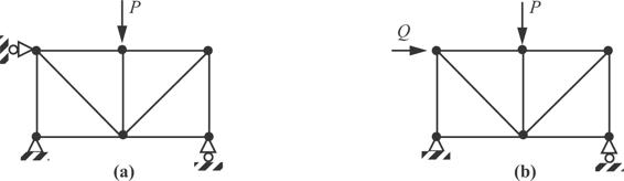— Fig. 6.17 A singly redundant truss (a), and its stable statically determinate base structure (b).

Example 6.8 Statically indeterminate truss

Consider the truss shown in part (a) of figure 6.18. The horizontal bars and the vertical bars have a length denoted by L, and each bar has the same elastic modulus E and same cross-sectional area A. For this truss m = 6, r = 3, and j = 4. So the truss is statically indeterminate. Note that this truss is statically determinate externally, but is statically indeterminate internally. Determine the bar forces in terms of the external applied load P.

A rectangular truss connects four corner nodes denoted 1 through 4, beginning at the bottom-left and moving counterclockwise around the structure. Each node is connected to the two adjacent to it, as well as to the one opposite it by a diagonal element. The top-left node 4 is pinned, but free to move in the vertical direction. The bottom-left node 1 is pinned and restricted in both displacements. An external force cap P is applied vertically at node 3. The same truss structure is used, but with the diagonal element between nodes 2 and 4 replaced by forces cap F sub 1 from node 2 and cap F sub 2 from node 4, both aligned with the previous diagonal element’s position and pointing inward towards one another. The previously removed diagonal element is now shown alone, with tensile forces cap Q on each end and aligned axially. 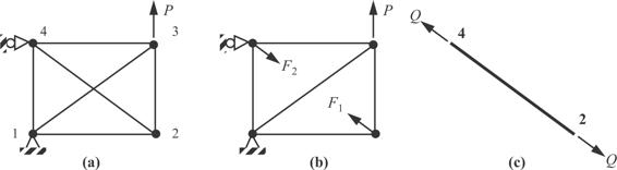— Fig. 6.18 (a) Statically indeterminate truss. (b) Statically determinant base structure with bar 2-4 replaced by forces F₁ and F₂. (c) Bar 2-4 subject to equal and opposite forces.

Solution. Consider a statically determinate truss with bar 2-4 removed, and a force F₁ acting at joint 2 and a force F₂ acting at joint 4 as shown in figure 6.18(b). These forces are oppositely directed along a line action coinciding with the removed bar 2-4. Let the complementary strain energy for this statically determinate, five-bar truss be denoted by Û^*. We employ Castigliano’s second theorem to determine the displacement u₁ corresponding to force F₁ and displacement u₂ corresponding to F₂. That is,

$\begin{align} u_{i} = \frac{\partial Û^{*}}{\partial F_{i}} = \frac{1}{E A} [L N_{12} \frac{\partial N_{12}}{\partial F_{i}} + \sqrt{2} L N_{13} \frac{\partial N_{13}}{\partial F_{i}} + L N_{14} \frac{\partial N_{14}}{\partial F_{i}} + L N_{23} \frac{\partial N_{23}}{\partial F_{i}} + L N_{34} \frac{\partial N_{34}}{\partial F_{i}}] i = 1, 2 . & (a) \end{align}$ $math-1161.png$

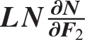
The bar forces are determined by joint equilibrium, and the results are shown in table 6.6. Bar forces are assumed positive in tension.

Table 6.6 Terms in eq. (a) for Castigliano’s second theorem

						$F_{1} = F_{2} = Q$ $math-1162.png$
Bar	Length L	Axial force N	∂N∕∂F₁	$L N \frac{\partial N}{\partial F_{1}}$ $math-1163.png$	$L N \frac{\partial N}{\partial F_{2}}$ $math-1164.png$	$L N \frac{\partial N}{\partial Q}$ $math-1165.png$
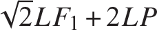
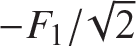
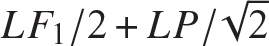
1-2	L	$- F_{1} / \sqrt{2}$ $math-1166.png$	$- 1 / \sqrt{2}$ $math-1167.png$	LF₁∕2	0	LQ∕2
1-3	$\sqrt{2} L$ $math-1168.png$	$F_{1} + \sqrt{2} P$ $math-1169.png$	1	$\sqrt{2} L F_{1} + 2 L P$ $math-1170.png$	0	$\sqrt{2} L Q + 2 L P$ $math-1171.png$
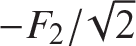
1-4	L	$- F_{2} / \sqrt{2}$ $math-1172.png$	0	0	(LF₂)∕2	(LQ)∕2
2-3	L	$- F_{1} / \sqrt{2}$ $math-1173.png$	$- 1 / \sqrt{2}$ $math-1174.png$	LF₁∕2	0	LQ∕2
3-4	L	$- F_{1} / \sqrt{2} - P$ $math-1175.png$	$- 1 / \sqrt{2}$ $math-1176.png$	$L F_{1} / 2 + L P / \sqrt{2}$ $math-1177.png$	0	$L Q / 2 + L P / \sqrt{2}$ $math-1178.png$

The sum of elements in column five divided by the product EA determines displacement u₁, and the sum of column six divided by EA determines u₂. Simplifying the results leads to

$\begin{align} u_{1} = \frac{L}{E A} [\frac{3 + 2 \sqrt{2}}{2}] F_{1} + \frac{L}{E A} [\frac{4 + \sqrt{2}}{2}] P and u_{2} = \frac{L}{2 E A} F_{2} . & (b) \end{align}$ $math-1179.png$

The relative inward displacement between joints 2 and joint 4 is given by the sum u₁ + u₂. For equal and opposite forces we set $F_{1} = F_{2} = Q$ $math-1180.png$ , and then the relative inward displacement reduces to

$\begin{align} Δ_{1 / 2} = u_{1} + {u_{2}|}_{F_{1} = F_{2} = Q} = \frac{L}{E A} [2 + \sqrt{2}] Q + \frac{L}{E A} [\frac{4 + \sqrt{2}}{2}] P . & (c) \end{align}$ $math-1181.png$

The seventh column in the table is obtained by setting $F_{1} = F_{2} = Q$ $math-1182.png$ . The sum of elements in the seventh column divided by EA is derivative of Û^* with respect to Q; i.e.,

$\begin{align} \frac{\partial Û^{*}}{\partial Q} = \frac{L}{E A} [2 + \sqrt{2}] Q + \frac{L}{E A} [\frac{4 + \sqrt{2}}{2}] P . & (d) \end{align}$ $math-1183.png$

We conclude that the relative inward displacement between joints 2 and joint 4 is given by

$\begin{align} Δ_{1 / 2} = \frac{\partial Û^{*}}{\partial Q} . & (e) \end{align}$ $math-1184.png$

The elongation of bar 2-4 is denoted by Δ₂₄ and its complementary strain energy is denoted by $U^{*}_{24}$ $math-1185.png$ . Hooke’s law for bar 2-4 is given by eq. (6.2) on page 144, which for N→Q and $L \to \sqrt{2} L$ $math-1186.png$ is solved for its elongation. The complementary strain energy is given by eq. (5.84) on page 136. These relations are

$\begin{align} Δ_{24} = \frac{\sqrt{2} L}{E A} Q and U_{24}^{*} = {\frac{1}{2 E A} \int_{0}^{\sqrt{2 L}} N^{2} d z|}_{N = Q} = \frac{\sqrt{2} L}{2 E A} Q^{2} . & (f) \end{align}$ $math-1187.png$

Castigliano’s second theorem is $\frac{\partial U^{*} 24}{\partial Q} = \frac{\sqrt{2} L}{E A} Q$ $math-1188.png$ , which is equal to the elongation. Thus, $Δ_{24} = \frac{\partial U_{24}^{*}}{\partial Q}$ $math-1189.png$ .

Geometric compatibility of the statically indeterminate, six-bar truss requires the relative inward displacement between joints 2 and 4 equals the negative of the elongation of bar 2-4. In other words, the sum $Δ_{1 / 2} + Δ_{24} = 0$ $math-1190.png$ . Hence,

$\begin{align} Δ_{1 / 2} + Δ_{24} = \frac{\partial Û^{*}}{\partial Q} + \frac{\partial U_{24}^{*}}{\partial Q} = \frac{\partial U^{*}}{\partial Q} = 0, & (g) \end{align}$ $math-1191.png$

where the total complementary strain energy of the statically indeterminate six-bar truss is $U^{*} = Û^{*} + U_{24}^{*}$ $math-1192.png$ . Hence, Castigliano’s second theorem applied to the six-bar truss is

$\begin{align} \frac{\partial U^{*}}{\partial Q} = \underset{\frac{\partial Û^{*}}{\partial Q}}{\underset{︸}{\frac{L}{E A} [2 + \sqrt{2}] Q + \frac{L}{E A} [\frac{4 + \sqrt{2}}{2}] P}} + \underset{\frac{\partial U^{*}_{24}}{\partial Q}}{\underset{︸}{\frac{\sqrt{2} L}{E A} Q}} = \frac{L}{E A} {2 (1 + \sqrt{2}) Q + [(4 + \sqrt{2}) P] / 2} = 0 . & (h) \end{align}$ $math-1193.png$

From eq. (h) we determine the redundant as

$\begin{align} Q = - (\frac{4 + \sqrt{2}}{4 (1 + \sqrt{2})}) P = - 0.56066 P . & (i) \end{align}$ $math-1194.png$

Finally, the bar forces are

$\begin{align} \begin{matrix} N_{1 - 2} = 0.396447 P & N_{1 - 3} = 0.853553 P & N_{1 - 4} = 0.396447 P \\ N_{2 - 3} = 0.396447 P & N_{2 - 4} = - 0.56066 P & N_{3 - 4} = - 0.603553 P \end{matrix} . & (j) \end{align}$ $math-1195.png$

The condition that $\partial U^{*} / \partial Q = 0$ $math-1196.png$ is interpreted as the relative displacement between the faces of an imaginary cut in bar 2-4 is equal to zero.

■

If the solution of the truss in example 6.8 was undertaken using Castigliano’s first theorem, it would lead to five simultaneous linear equations for the unknown joint displacements $q_{3}, q_{4}, q_{5}, q_{6}$ $math-1197.png$ , and, q₈ in terms of the applied load P. (Refer to “Coplanar trusses” on page 143 for the displacement numbering convention.) After solving for these simultaneous equations for the joints displacements, the elongations of each bar, Δ_i − j, would be computed from eq. (6.6) on page 145. Lastly, the bar forces are determined from $N_{i - j} = {(E A / L)}_{i - j} Δ_{i - j}$ $math-1198.png$ . Using Castigliano’s second theorem for this singly redundant truss, we only had to solve one equation for the unknown redundant Q. The number of simultaneous equations to be solved in a statically indeterminate structure by Castigliano’s second theorem is equal to the number of redundants.

Example 6.9 King Post truss

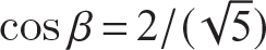
In this example we paraphrase the problem statement given in the text by Bruhn (1973, p. A8.42). The structure shown in figure 6.19 consists of members ADC, AB, BC, and BD. Continuous member ADC is simply supported at ends A and C, has an area of 9.25 in², and a second area moment of 216 in⁴. Members AB, BC and BD have areas of 2 in². The modulus of elasticity is the same for all members. Determine the internal actions in each member using Castigliano’s second theorem.

A horizontal beam element, 240 inches in length, is pinned at each end, denoted cap A on the left end and cap C on the right end, but is free to displace in the horizontal direction. Point cap D is at the center of the beam as is where an external load of 5000 pounds is applied downward. A vertical bar element connects points cap D and cap B, and is 60 inches in length. Two diagonal bar elements connect point cap B with both cap A and cap C, each resulting in the formation of triangle with a width of 120 inches and a height of 60 inches. — Fig. 6.19 King post truss.

Solution. This structure is statically determinant externally. Also, the structure, its support conditions, and the external loading are symmetric about the vertical line of action of the 5,000 lb. force. The support reactions of the truss removed from its supports at A and C are shown in figure 6.20(a). Consideration of the free body diagrams of members AD, AB, and BD in figure 6.20(b) leads to the conclusion that this structure is statically indeterminate internally. The redundant Q is taken as the axial force in member AB. If Q is known, then the forces and moments in the other members are determined by equilibrium. Neglecting the energy due to transverse shear in member ADC, the complementary strain energy is

The same combination of beam and bar elements is shown, but with the pins at cap A and cap C now replaced by reaction forces cap P over 2. Additionally, the lengths have been replaced with general length cap L, as well as the height of the cap D cap B member being denoted cap L over 2. The external force at cap D has been generalized to magnitude cap P downward. The bars connecting cap A or cap C to cap B, are also shown to make an angle beta with the horizontal beam element. The previous structure is now separated into three parts. The horizontal beam element originating at cap A is given a local coordinate frame at cap A, with z aligned with the beam, while y is normal upwards. The beam experiences reaction load cap P over 2 vertically at cap A, as well as an internal load cap Q oriented to the right and downward at an angle beta to the horizontal. At point z along the beam, internal forces are shown with cap N denoting axial loading, cap V upwards denoting shear force, and clockwise moment cap M. These expressions are only valid for z values between 0 and cap L. The bar between cap A and cap B is shown, with tensile forces cap Q at each end. Member cap B cap D is shown with two cap Q forces pointing up and away from point cap B on both sides, each at angle beta to the horizontal. An axial tension force cap N sub cap B cap D is also shown within the bar. 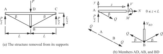— Fig. 6.20 Free body diagrams of the king post truss.

$\begin{align} U^{*} = 2 \int_{0}^{L} [\frac{N^{2}}{2 E A_{A C}} + \frac{M^{2}}{2 E I}] d z + 2 [\frac{L_{A B} Q^{2}}{2 E A}] + \frac{(L / 2) N_{B D}^{2}}{2 E A} . & (a) \end{align}$ $math-1199.png$

Note that the complementary strain energy in members AD and AB are multiplied by two to account for the energy in members DC and BC, respectively. The compatibility condition that the relative displacement of an imaginary cut in member AB vanishes is that the derivative of the complementary energy with respect to Q equals zero. Thus,

$\begin{align} 0 = 2 \int_{0}^{L} \{\frac{N}{E A_{A C}} (\frac{\partial N}{\partial Q}) + \frac{M}{E I} (\frac{\partial M}{\partial Q})\} d z + \frac{2 L_{A B} Q}{E A} + \frac{(L / 2) N_{B D}}{E A} (\frac{\partial N_{A B}}{\partial Q}) . & (b) \end{align}$ $math-1200.png$

Equilibrium equations of member AD are

$\begin{align} N + Q cos β = 0 V + P / 2 - Q sin β = 0 M + (P / 2 - Q sin β) z = 0 0 \leq z < L . & (c) \end{align}$ $math-1201.png$

The axial equilibrium equation for member BD is

$\begin{align} N_{B D} + 2 Q sin β = 0 . & (d) \end{align}$ $math-1202.png$

Substitute member axial forces and moment from the equilibrium eq. (c) into the compatibility condition (b) to get

$\begin{align} 0 = 2 \int_{0}^{L} \{\frac{(- Q cos β)}{E A_{A C}} (- cos β) + \frac{[- (P / 2 - Q sin β) z]}{E I} [(sin β) z]\} d z + \frac{2 L_{A B} Q}{E A} + \frac{(L / 2) (- 2 Q sin β)}{E A} (- 2 sin β) . & (e) \end{align}$ $math-1203.png$

Perform the integration in eq. (e) followed by the substitutions $L_{A B} = (\sqrt{5} L) / 2$ $math-1204.png$ , $cos β = 2 / (\sqrt{5})$ $math-1205.png$ , and $sin β = 1 / (\sqrt{5})$ $math-1206.png$ to find

$\begin{align} 0 = 2 (\frac{- L^{3} P}{6 \sqrt{5} E I} + \frac{4 L Q}{5 E A_{A C}} + \frac{L^{3} Q}{15 E I}) + \frac{2 L Q}{5 E A} + \frac{\sqrt{5} L Q}{E A} . & (f) \end{align}$ $math-1207.png$

Solve. (f) for the redundant Q:

$\begin{align} Q = \frac{\sqrt{5} A A_{A C} L^{2} P}{24 A I + 6 A_{A C} I + 15 \sqrt{5} A_{A C} I + 2 A A_{A C} L^{2}} . & (g) \end{align}$ $math-1208.png$

Substitute the numerical values for the quantities on the right-hand side of eq. (g) to find the redundant:

$\begin{align} Q = \frac{\sqrt{5} (2) (9.25) (12 0^{2}) (5000)}{24 (2) (216) + 6 (9.25) (216) + 15 \sqrt{5} (9.25) (216) + 2 (2) (9.25) (12 0^{2})} = 4, 787.18 lb . & (h) \end{align}$ $math-1209.png$

The axial force in member BD from eq. (d) is

$N_{B D} = - 2 (4787.18) (\frac{1}{\sqrt{5}}) = - 4281.78 lb .$ $math-1210.png$

The negative value of N_BD means member BD is in compression. The axial force and bending moment in member AD is

$\begin{align} N = - (4787.18) 2 / \sqrt{5} = - 4281.78 lb . M = (- 2500 + \frac{(4787.18)}{\sqrt{5}}) z = (- 359.11 lb .) z 0 \leq z < 120 in. & (i) \end{align}$ $math-1211.png$

■

Search

Text Color

Text Size

Margin Size

Font Type

6.4 Castigliano’s second theorem and statically indeterminate structures