18.10: References

Last updated
Save as PDF

Page ID: 95342

$ \newcommand{\vecs}[1]{\overset { \scriptstyle \rightharpoonup} {\mathbf{#1}} } $

$ \newcommand{\vecd}[1]{\overset{-\!-\!\rightharpoonup}{\vphantom{a}\smash {#1}}} $

$ \newcommand{\id}{\mathrm{id}}$ $ \newcommand{\Span}{\mathrm{span}}$

( \newcommand{\kernel}{\mathrm{null}\,}\) $ \newcommand{\range}{\mathrm{range}\,}$

$ \newcommand{\RealPart}{\mathrm{Re}}$ $ \newcommand{\ImaginaryPart}{\mathrm{Im}}$

$ \newcommand{\Argument}{\mathrm{Arg}}$ $ \newcommand{\norm}[1]{\| #1 \|}$

$ \newcommand{\inner}[2]{\langle #1, #2 \rangle}$

$ \newcommand{\Span}{\mathrm{span}}$

$ \newcommand{\id}{\mathrm{id}}$

$ \newcommand{\Span}{\mathrm{span}}$

$ \newcommand{\kernel}{\mathrm{null}\,}$

$ \newcommand{\range}{\mathrm{range}\,}$

$ \newcommand{\RealPart}{\mathrm{Re}}$

$ \newcommand{\ImaginaryPart}{\mathrm{Im}}$

$ \newcommand{\Argument}{\mathrm{Arg}}$

$ \newcommand{\norm}[1]{\| #1 \|}$

$ \newcommand{\inner}[2]{\langle #1, #2 \rangle}$

$ \newcommand{\Span}{\mathrm{span}}$ $ \newcommand{\AA}{\unicode[.8,0]{x212B}}$

$ \newcommand{\vectorA}[1]{\vec{#1}} % arrow$

$ \newcommand{\vectorAt}[1]{\vec{\text{#1}}} % arrow$

$ \newcommand{\vectorB}[1]{\overset { \scriptstyle \rightharpoonup} {\mathbf{#1}} } $

$ \newcommand{\vectorC}[1]{\textbf{#1}} $

$ \newcommand{\vectorD}[1]{\overrightarrow{#1}} $

$ \newcommand{\vectorDt}[1]{\overrightarrow{\text{#1}}} $

$ \newcommand{\vectE}[1]{\overset{-\!-\!\rightharpoonup}{\vphantom{a}\smash{\mathbf {#1}}}} $

$ \newcommand{\vecs}[1]{\overset { \scriptstyle \rightharpoonup} {\mathbf{#1}} } $

$ \newcommand{\vecd}[1]{\overset{-\!-\!\rightharpoonup}{\vphantom{a}\smash {#1}}} $

$\newcommand{\avec}{\mathbf a}$ $\newcommand{\bvec}{\mathbf b}$ $\newcommand{\cvec}{\mathbf c}$ $\newcommand{\dvec}{\mathbf d}$ $\newcommand{\dtil}{\widetilde{\mathbf d}}$ $\newcommand{\evec}{\mathbf e}$ $\newcommand{\fvec}{\mathbf f}$ $\newcommand{\nvec}{\mathbf n}$ $\newcommand{\pvec}{\mathbf p}$ $\newcommand{\qvec}{\mathbf q}$ $\newcommand{\svec}{\mathbf s}$ $\newcommand{\tvec}{\mathbf t}$ $\newcommand{\uvec}{\mathbf u}$ $\newcommand{\vvec}{\mathbf v}$ $\newcommand{\wvec}{\mathbf w}$ $\newcommand{\xvec}{\mathbf x}$ $\newcommand{\yvec}{\mathbf y}$ $\newcommand{\zvec}{\mathbf z}$ $\newcommand{\rvec}{\mathbf r}$ $\newcommand{\mvec}{\mathbf m}$ $\newcommand{\zerovec}{\mathbf 0}$ $\newcommand{\onevec}{\mathbf 1}$ $\newcommand{\real}{\mathbb R}$ $\newcommand{\twovec}[2]{\left[\begin{array}{r}#1 \\ #2 \end{array}\right]}$ $\newcommand{\ctwovec}[2]{\left[\begin{array}{c}#1 \\ #2 \end{array}\right]}$ $\newcommand{\threevec}[3]{\left[\begin{array}{r}#1 \\ #2 \\ #3 \end{array}\right]}$ $\newcommand{\cthreevec}[3]{\left[\begin{array}{c}#1 \\ #2 \\ #3 \end{array}\right]}$ $\newcommand{\fourvec}[4]{\left[\begin{array}{r}#1 \\ #2 \\ #3 \\ #4 \end{array}\right]}$ $\newcommand{\cfourvec}[4]{\left[\begin{array}{c}#1 \\ #2 \\ #3 \\ #4 \end{array}\right]}$ $\newcommand{\fivevec}[5]{\left[\begin{array}{r}#1 \\ #2 \\ #3 \\ #4 \\ #5 \\ \end{array}\right]}$ $\newcommand{\cfivevec}[5]{\left[\begin{array}{c}#1 \\ #2 \\ #3 \\ #4 \\ #5 \\ \end{array}\right]}$ $\newcommand{\mattwo}[4]{\left[\begin{array}{rr}#1 \amp #2 \\ #3 \amp #4 \\ \end{array}\right]}$ $\newcommand{\laspan}[1]{\text{Span}\{#1\}}$ $\newcommand{\bcal}{\cal B}$ $\newcommand{\ccal}{\cal C}$ $\newcommand{\scal}{\cal S}$ $\newcommand{\wcal}{\cal W}$ $\newcommand{\ecal}{\cal E}$ $\newcommand{\coords}[2]{\left\{#1\right\}_{#2}}$ $\newcommand{\gray}[1]{\color{gray}{#1}}$ $\newcommand{\lgray}[1]{\color{lightgray}{#1}}$ $\newcommand{\rank}{\operatorname{rank}}$ $\newcommand{\row}{\text{Row}}$ $\newcommand{\col}{\text{Col}}$ $\renewcommand{\row}{\text{Row}}$ $\newcommand{\nul}{\text{Nul}}$ $\newcommand{\var}{\text{Var}}$ $\newcommand{\corr}{\text{corr}}$ $\newcommand{\len}[1]{\left|#1\right|}$ $\newcommand{\bbar}{\overline{\bvec}}$ $\newcommand{\bhat}{\widehat{\bvec}}$ $\newcommand{\bperp}{\bvec^\perp}$ $\newcommand{\xhat}{\widehat{\xvec}}$ $\newcommand{\vhat}{\widehat{\vvec}}$ $\newcommand{\uhat}{\widehat{\uvec}}$ $\newcommand{\what}{\widehat{\wvec}}$ $\newcommand{\Sighat}{\widehat{\Sigma}}$ $\newcommand{\lt}{<}$ $\newcommand{\gt}{>}$ $\newcommand{\amp}{&}$ $\definecolor{fillinmathshade}{gray}{0.9}$

18.10 References

Bathe, K-L. Finite Element Procedures in Engineering Analysis. Englewood Cliffs, NJ: Prentice-Hall Inc., 1982.
Boresi, A. P. Elasticity In Engineering Mechanics. Englewood Cliffs, N.J: Prentice-Hall, Inc. 1965, p. 34.
Craig, Roy R., Jr. Structural Dynamics: An Introduction to Computer Methods. New York: John Wiley & Sons, Inc., 1981, pp. 212–217, 321–340, 455–464.
Hallauer, W. L., Jr., Introduction to Linear, Time-Invariant, Dynamic Systems for Students of Engineering. Blacksburg, VA: Self-published, 2016. http://hdl.handle.net/10919/78864.
Isakowitz, Steven J. Space Launch Systems, 2d ed. Updated by Jeff Samella.Washington DC: American Institute of Aeronautics and Astronautics, 1995, pp. 201–218.
Langhaar, H. L. Energy Methods in Applied Mechanics. New York: John Wiley, and Sons, Inc., 1962.
Qu, Zu-Qing. Model Order Reduction Techniques, With Application to Finite Element Analysis. London: Springer-Verlag, 2004.
Sarafin, Thomas, P., ed. Spacecraft Structures and Mechanisms - From Concept to Launch. Torrance, CA, and Dordrecht, The Netherlands: Microcosom Press, and Kluwer, 1995, pp. 49 & 50.
Schiesser, W. E. Computational Mathematics in Engineering and Applied Science. Boca Raton, FL: CRC Press, 1994, Chapter 2.
Szabó, B., and I. Babuska. Finite Element Analysis. New York: John Wiley & Sons, 1991, pp. 163–166.

18.11 Practice exercises

1. The Lagrangian for a three-degree-of-freedom model of Atlas I is

$\begin{align} L = \frac{m_{1}}{6} [{(ẇ_{1})}^{2} + ẇ_{} 1 ẇ_{2} + {(ẇ_{2})}^{2}] + 12 m_{2} {(ẇ_{2})}^{2} + 12 m_{3} {(ẇ_{3})}^{2} - 12 k_{12} {(w_{1} - w_{2})}^{2} - 12 k_{23} {(w_{3} - w_{2})}^{2}, & (18.196) \end{align}$ $math-4388.png$

where w₁(t) is the displacement at the bottom of the booster, w₂(t) is the displacement at the top of Centaur, and w₃(t) is the displacement of the payload. These displacements are defined with respect to the equilibrium state. The combined mass of the booster and Centaur is denoted by m₁, the mass of the fairing by m₂, and the mass of the payload by m₃. Masses are determined from the weight data given in “Description of Atlas I” on page 485. The spring stiffness k₁₂ and k₂₃ are listed in “Step 1: Equations of motion about equilibrium.” on page 488. Lagrange’s equations of motion are

$\begin{align} \frac{d}{d t} (\frac{\partial L}{\partial ẇ_{1}}) - \frac{\partial L}{\partial w_{1}} = R_{1} \frac{d}{d t} (\frac{\partial L}{\partial ẇ_{2}}) - \frac{\partial L}{\partial w_{2}} = 0 \frac{d}{d t} (\frac{\partial L}{\partial ẇ_{3}}) - \frac{\partial L}{\partial w_{3}} = 0, & (18.197) \end{align}$ $math-4389.png$

where $R_{1} = 77, 100$ $math-4390.png$ . lb is the net thrust. Determine the maximum payload load factor during the initial instants of lift off. Partial answer: the value and its associated eigenvector for the smallest elastic mode is

$\begin{align} (λ_{2}, \{ϕ_{2}\}) = (15, 710.5, [\begin{matrix} - 0.795164 \\ 0.760969 \\ 1 \end{matrix}]) . & (18.198) \end{align}$ $math-4391.png$

The eigenvector is normalized such that the magnitude of its largest component is a positive one.

2. Determine the natural frequencies in Hz and the corresponding modal vectors for the five-bar, pin-jointed truss shown in figure 18.24. Normalize the modal vectors such that the largest component in the vector is a positive 1. Sketch the mode shapes.

A 5 bar truss connects four nodes in the shape of a rectangle. Node 1 is the bottom right corner, with the numbers increasing in a counterclockwise rotation to node 4 at the bottom left corner. Nodes 2 and 3 are 4 meters directly above nodes 1 and 4, which are 3 meters apart. Each node is connected to the other three, with the exception of nodes 3 and 4 not being connected to one another. Instead, they are pinned to a wall. Each node has two degrees of freedom, horizontal and vertical displacement. The horizontal displacements are the odd degrees of freedom, while the vertical displacements are the even degrees of freedom, with the numbers increasing in the same pattern as the nodes. All bars have Young’s Modulus of 70 gigapascals, Area of 475 times 10 to the negative 6 meters squared, and density of 2710 kilograms per cubic meter. 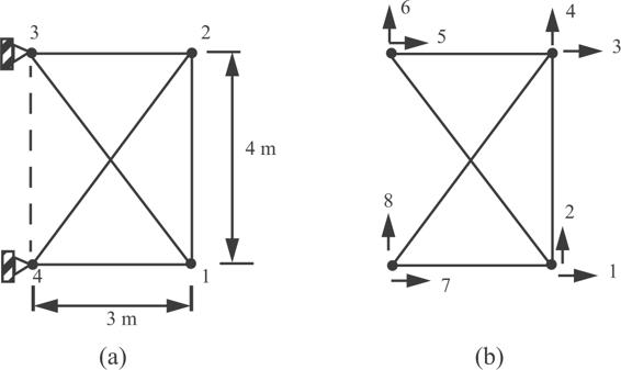— Fig. 18.24 (a) Five-bar truss, (b) Degrees of freedom.

3. The three-bar truss in example 18.3 on page 511 is subjected to the following initial conditions

$\begin{align} [\begin{matrix} u_{1} (0) \\ u_{2} (0) \end{matrix}] = {[\begin{matrix} 0 \\ 0 \end{matrix}] [\begin{matrix} \frac{d u_{1}}{d t} \\ \frac{d u_{2}}{d t} \end{matrix}]|}_{t = 0} = [\begin{matrix} 0 \\ 1 \end{matrix}] m / s . & (18.199) \end{align}$ $math-4392.png$

a) Determine the generalized mass matrix [M_g], the generalized stiffness matrix [K_g], and the initial conditions in modal coordinates (begin with eqs. (d) and (e)).

b) Determine the solution in modal coordinates and in physical coordinates.

c) Determine the transient bar forces $N_{1 - 2} (t), N_{1 - 3} (t), and N_{1 - 4} (t)$ $math-4393.png$ .

d) Plot the bar forces found in part (c) for $0 \leq t \leq 0.015 s$ $math-4394.png$ .

4. Model the cantilever beam in example 18.4 on page 518 with two equal length elements as shown in figure 18.25.

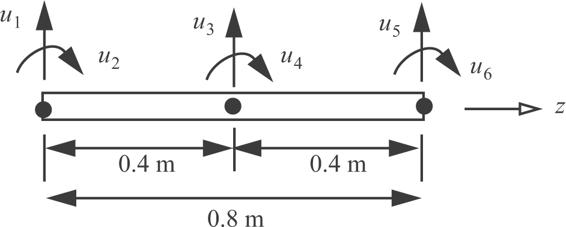
A 2 meter long beam is divided into two halves by a set of 3 nodes, one at each end and one in the center. The vertical displacements are numbered u sub 1, u sub 3, and u sub 5, for the left, center, and right nodes, respectively. The rotations are denoted by u sub 2, u sub 4, and u sub 6 for the left, center, and right nodes, respectively. — Fig. 18.25 Beam of example 18.4 modeled with two elements.

a) Determine the natural frequencies in Hz and the corresponding modal vectors. Normalize the modal vectors such that the tip displacement u₅ is equal to one in each mode. Refer to table 18.4.

b) Determine the percentage error of each frequency with respect to the exact frequency from the continuous beam vibration analysis.

c) Plot the lateral displacement of the beam, $0 \leq z \leq 0.8 m$ $math-4395.png$ , for each mode using eq. (17.69) on page 463 and matrix [G_aq] from the last three rows of eq. (18.162).

5. The uniform beam shown in figure 18.26 is simply supported at each end. The material and geometric properties are the same as those given in example 18.4,

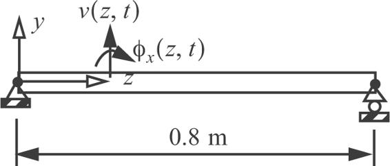
A 2 meter long beam is pinned at both ends, with the z axis aligned with the beam’s length and y normal to the beam length upwards, both centered at the left pinned edge. Vertical displacement is denoted by v as a function of z and t. Cap E cap I is 132209 Newtons times square meters, cap A is 475 times 10 to the negative 6 square meters, and rho is 2710 kilograms per cubic meter. — Fig. 18.26 Simply supported beam.

a. Determine the first two natural frequencies in Hz for the beam modeled with one element. Use the condensed mass matrix (18.167) and stiffness matrix (17.106) on page 468.

b. Compute the percent discrepancy of the frequencies with respect to the continuous beam solution. The frequencies for the continuous beam vibration analysis in rad/s are listed in Graig (1981) as $ω_{n} = (\frac{n π}{l}) 2 \sqrt{E I_{x x}} \sqrt{\frac{}{ρ A}}$ $math-4396.png$ $n = 1, 2$ $math-4397.png$ .

1. Requirements for generalized coordinates are (1) that there is a one-to-one correspondence between the coordinates and the configuration of the mechanical system, and (2) that infinitesimal increments in the generalized coordinates result in infinitesimal increments in the configuration. Requirement (1) precludes constraint equations between the generalize coordinates.

Search

Text Color

Text Size

Margin Size

Font Type

18.10 References

18.11 Practice exercises