
3.7: Light Scattering by a Slit
- Page ID
- 10106

\( \newcommand{\vecs}[1]{\overset { \scriptstyle \rightharpoonup} {\mathbf{#1}} } \)
\( \newcommand{\vecd}[1]{\overset{-\!-\!\rightharpoonup}{\vphantom{a}\smash {#1}}} \)
\( \newcommand{\dsum}{\displaystyle\sum\limits} \)
\( \newcommand{\dint}{\displaystyle\int\limits} \)
\( \newcommand{\dlim}{\displaystyle\lim\limits} \)
\( \newcommand{\id}{\mathrm{id}}\) \( \newcommand{\Span}{\mathrm{span}}\)
( \newcommand{\kernel}{\mathrm{null}\,}\) \( \newcommand{\range}{\mathrm{range}\,}\)
\( \newcommand{\RealPart}{\mathrm{Re}}\) \( \newcommand{\ImaginaryPart}{\mathrm{Im}}\)
\( \newcommand{\Argument}{\mathrm{Arg}}\) \( \newcommand{\norm}[1]{\| #1 \|}\)
\( \newcommand{\inner}[2]{\langle #1, #2 \rangle}\)
\( \newcommand{\Span}{\mathrm{span}}\)
\( \newcommand{\id}{\mathrm{id}}\)
\( \newcommand{\Span}{\mathrm{span}}\)
\( \newcommand{\kernel}{\mathrm{null}\,}\)
\( \newcommand{\range}{\mathrm{range}\,}\)
\( \newcommand{\RealPart}{\mathrm{Re}}\)
\( \newcommand{\ImaginaryPart}{\mathrm{Im}}\)
\( \newcommand{\Argument}{\mathrm{Arg}}\)
\( \newcommand{\norm}[1]{\| #1 \|}\)
\( \newcommand{\inner}[2]{\langle #1, #2 \rangle}\)
\( \newcommand{\Span}{\mathrm{span}}\) \( \newcommand{\AA}{\unicode[.8,0]{x212B}}\)
\( \newcommand{\vectorA}[1]{\vec{#1}} % arrow\)
\( \newcommand{\vectorAt}[1]{\vec{\text{#1}}} % arrow\)
\( \newcommand{\vectorB}[1]{\overset { \scriptstyle \rightharpoonup} {\mathbf{#1}} } \)
\( \newcommand{\vectorC}[1]{\textbf{#1}} \)
\( \newcommand{\vectorD}[1]{\overrightarrow{#1}} \)
\( \newcommand{\vectorDt}[1]{\overrightarrow{\text{#1}}} \)
\( \newcommand{\vectE}[1]{\overset{-\!-\!\rightharpoonup}{\vphantom{a}\smash{\mathbf {#1}}}} \)
\( \newcommand{\vecs}[1]{\overset { \scriptstyle \rightharpoonup} {\mathbf{#1}} } \)
\(\newcommand{\longvect}{\overrightarrow}\)
\( \newcommand{\vecd}[1]{\overset{-\!-\!\rightharpoonup}{\vphantom{a}\smash {#1}}} \)
\(\newcommand{\avec}{\mathbf a}\) \(\newcommand{\bvec}{\mathbf b}\) \(\newcommand{\cvec}{\mathbf c}\) \(\newcommand{\dvec}{\mathbf d}\) \(\newcommand{\dtil}{\widetilde{\mathbf d}}\) \(\newcommand{\evec}{\mathbf e}\) \(\newcommand{\fvec}{\mathbf f}\) \(\newcommand{\nvec}{\mathbf n}\) \(\newcommand{\pvec}{\mathbf p}\) \(\newcommand{\qvec}{\mathbf q}\) \(\newcommand{\svec}{\mathbf s}\) \(\newcommand{\tvec}{\mathbf t}\) \(\newcommand{\uvec}{\mathbf u}\) \(\newcommand{\vvec}{\mathbf v}\) \(\newcommand{\wvec}{\mathbf w}\) \(\newcommand{\xvec}{\mathbf x}\) \(\newcommand{\yvec}{\mathbf y}\) \(\newcommand{\zvec}{\mathbf z}\) \(\newcommand{\rvec}{\mathbf r}\) \(\newcommand{\mvec}{\mathbf m}\) \(\newcommand{\zerovec}{\mathbf 0}\) \(\newcommand{\onevec}{\mathbf 1}\) \(\newcommand{\real}{\mathbb R}\) \(\newcommand{\twovec}[2]{\left[\begin{array}{r}#1 \\ #2 \end{array}\right]}\) \(\newcommand{\ctwovec}[2]{\left[\begin{array}{c}#1 \\ #2 \end{array}\right]}\) \(\newcommand{\threevec}[3]{\left[\begin{array}{r}#1 \\ #2 \\ #3 \end{array}\right]}\) \(\newcommand{\cthreevec}[3]{\left[\begin{array}{c}#1 \\ #2 \\ #3 \end{array}\right]}\) \(\newcommand{\fourvec}[4]{\left[\begin{array}{r}#1 \\ #2 \\ #3 \\ #4 \end{array}\right]}\) \(\newcommand{\cfourvec}[4]{\left[\begin{array}{c}#1 \\ #2 \\ #3 \\ #4 \end{array}\right]}\) \(\newcommand{\fivevec}[5]{\left[\begin{array}{r}#1 \\ #2 \\ #3 \\ #4 \\ #5 \\ \end{array}\right]}\) \(\newcommand{\cfivevec}[5]{\left[\begin{array}{c}#1 \\ #2 \\ #3 \\ #4 \\ #5 \\ \end{array}\right]}\) \(\newcommand{\mattwo}[4]{\left[\begin{array}{rr}#1 \amp #2 \\ #3 \amp #4 \\ \end{array}\right]}\) \(\newcommand{\laspan}[1]{\text{Span}\{#1\}}\) \(\newcommand{\bcal}{\cal B}\) \(\newcommand{\ccal}{\cal C}\) \(\newcommand{\scal}{\cal S}\) \(\newcommand{\wcal}{\cal W}\) \(\newcommand{\ecal}{\cal E}\) \(\newcommand{\coords}[2]{\left\{#1\right\}_{#2}}\) \(\newcommand{\gray}[1]{\color{gray}{#1}}\) \(\newcommand{\lgray}[1]{\color{lightgray}{#1}}\) \(\newcommand{\rank}{\operatorname{rank}}\) \(\newcommand{\row}{\text{Row}}\) \(\newcommand{\col}{\text{Col}}\) \(\renewcommand{\row}{\text{Row}}\) \(\newcommand{\nul}{\text{Nul}}\) \(\newcommand{\var}{\text{Var}}\) \(\newcommand{\corr}{\text{corr}}\) \(\newcommand{\len}[1]{\left|#1\right|}\) \(\newcommand{\bbar}{\overline{\bvec}}\) \(\newcommand{\bhat}{\widehat{\bvec}}\) \(\newcommand{\bperp}{\bvec^\perp}\) \(\newcommand{\xhat}{\widehat{\xvec}}\) \(\newcommand{\vhat}{\widehat{\vvec}}\) \(\newcommand{\uhat}{\widehat{\uvec}}\) \(\newcommand{\what}{\widehat{\wvec}}\) \(\newcommand{\Sighat}{\widehat{\Sigma}}\) \(\newcommand{\lt}{<}\) \(\newcommand{\gt}{>}\) \(\newcommand{\amp}{&}\) \(\definecolor{fillinmathshade}{gray}{0.9}\)One of the most spectacular successes for phasor analysis arises in the study of light diffraction by a narrow slit. The experiment is to shine laser light through a slit in an otherwise opaque sheet and observe the pattern of light that falls on a distant screen. When the slit is very narrow compared with the wavelength of the light, then the light that falls on the screen is nearly uniform in intensity. However, when the width of the slit is comparable to the wavelength of the light, the pattern of light that falls on the screen is scalloped in intensity, showing alternating light and dark bands. The experiment, and the observed results, are illustrated in the Figure.
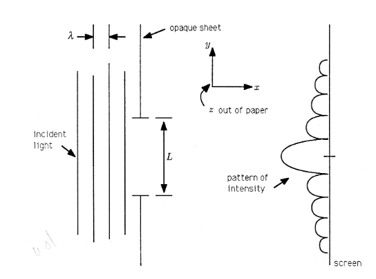
Why should this experiment produce this result? Phasor analysis illuminates the question and produces an elegant mathematical description of a profoundly important optical experiment.
Huygens's Principle
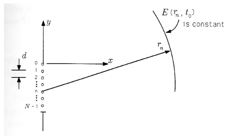
We will assume, as Christiaan Huygens did, that the light incident on the slit sets up a light field in the slit that may be modeled by \(N\) discrete sources, each of which radiates a “spherical wave of light.” This model is illustrated in the Figure. The distance between sources is \(d\), and \(Nd=L\) is the width of the slit. Each source is indexed by \(n\), and \(n\) runs from 0 to \(N−1\). The 0th source is located at the origin of our coordinate system.
The spherical wave radiated by the \(n^{\mathrm{th}}\) source is described by the equation
\[E(r_n,t)=\mathrm{Re}\{\frac A N e^{j[ωt−(2π/λ)r_n]}\} \nonumber \]
The function \(E(r_n,t)\) describes the “electric field” at time \(t\) and distance \(r_n\) from the \(n^\mathrm{th}\) source. The field is constant as long as the variable \(ωt−(2π/λ)r_n\) is constant. Therefore, if we freeze time at \(t=t_0\), the field will be constant on a sphere of radius \(r_n\). This is illustrated in the Figure.
Fix \(r_n\) in \(E(r_n,t)\) and show that \(E(r_n,t)\) varies cosinusoidally with time \(t\). Sketch the function and interpret it. What is its period?
Fix \(t\) in \(E(r_n,t)\) and show that \(E(r_n,t)\) varies cosinusoidally with radius \(r_n\). Sketch the function and interpret it. Call the “period in \(r_n\)" the “wavelength.” Show that the wavelength is \(λ\).
The “crest of the wave \(E(r_n,t)\)" occurs when \(ωt−(2π/λ)r_n=0\). Show that the crest moves through space at velocity \(v=ωλ/2π\).
Geometry
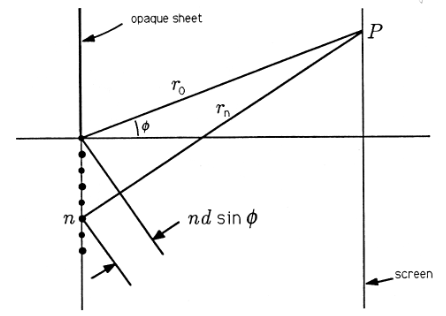
If we now pick a point \(P\) on a distant screen, that point will be at distance \(r_0\) from source 0,...,\(r_n\) from source \(n\),..., and so on. If we isolate the sources 0 and \(n\), then we have the geometric picture of the Figure. The angle \(φ\) is the angle that point \(P\) makes with the horizontal axis. The Pythagorean theorem says that the connection between distances \(r_0\) and \(r_n\) is
\[(r_n−nd\sinφ)^2+(nd\cosφ)^2=r^2_0 \nonumber \]
Let's try the solution
\[r_n=r_0+nd\sinφ \nonumber \]
This solution produces the approximate identity
\[r^2_0+(nd\cosφ)^2≅r^2_0 \nonumber \]
\[r^2_0+(nd\cosφ)^2≅r^2_0 \nonumber \]
\[1+(\frac {nd} {r_0} \cosφ)^2≅1 \nonumber \]
This will be close for \(\frac {nd} {r_0} <<1\). We will assume that the slit width \(L\) is small compared to the distance to any point on the screen.
Then \(\frac {Nd} {r_0} = \frac {L} {r_0} << 1\), in which case the approximate solution for \(r_n\) is valid for all \(n\). This means that, for any point \(P\) on the distant screen, the light contributed by the \(n^{th}\) source is approximately
\[E_n(φ,t)=\mathrm{Re}\{\frac A N e^{j[ωt−(2π/λ)(r_0+nd\sinφ)]}\}=\mathrm{Re}\{\frac A N e^{−j(2π/λ)r_0}e^{−j(2π/λ)nd\sinφ}e^{jωt}\} \nonumber \]
The phasor representation for this function is just
\[E_n(φ)=\frac A N e^{−j(2π/λ)r_0} e^{−j(2π/λ)nd\sinφ} \nonumber \]
Note that \(E_0(φ)\), the phasor associated with the 0th source, is \(\frac A N e^{−j(2π/λ)r_0}\). Therefore we may write the phasor representation for the light contributed by the \(n^{th}\) source to be
\[E_n(φ)=E_0(φ)e^{−j(2π/λ)nd\sinφ} \nonumber \]
This result is very important because it shows the light arriving at point \(P\) from different sources to be “out of phase” by an amount that depends on the ratio \(\frac {nd\sinφ} λ\)
Phasors and Interference
The phasor representation for the field observed at point \(P\) on the screen is the sum of the phasors contributed by each source:
\[E(φ)=∑_{n=0}^{N−1} E_n(φ)=E_0(φ)∑_{n=0}^{N−1}e^{−j(2π/λ)nd\sinφ} \nonumber \]
This is a sum of the form
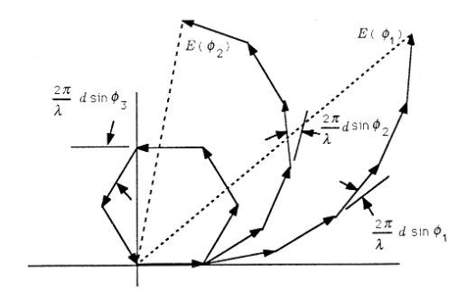
\[E(φ)=E_0(φ)∑_{n=0}^{N−1}e^{jnθ} \nonumber \]
where the angle \(θ\) is \((2π/λ)d\sinφ\). This sum is illustrated in the Figure for several representative values of \(θ\). Note that for small \(θ\), meaning small \(φ\), the sum has large magnitude, whereas for \(θ\) on the order of \(2π/N\), the sum is small. This simple geometric interpretation shows that for some values of \(φ\), corresponding to some points \(P\) on the screen, there will be constructive interference between the phasors, while for other values of \(φ\) there will be destructive interference. Constructive interference produces bright light, and destructive interference produces darkness.
The geometry of the Figure is illuminating. However, we already know from our study of complex numbers and geometric sums that the phasor sum of the Equation may be written as
\[E(φ)=E_0(φ)\frac {1−e^{−j(2π/λ)Nd\sinφ}} {1−e^{−j(2π/λ)d\sinφ}} \nonumber \]
This result may be manipulated to produce the form
\[E(φ)=\frac A N e^{−j(2π/λ)r_0} e^{−j(π/λ)(N−1)d\sinφ}\frac {\sin(Nπ\frac d λ \sinφ)} {\sin(π\frac d λ \sinφ)} \nonumber \]
The magnitude is the intensity of the light at angle \(φ\) from horizontal:
\[|E(φ)|=|\frac A N \frac {\sin(Nπ\frac d λ \sinφ)} {\sin(π\frac d λ \sinφ)}| \nonumber \]
Derive \(\frac A N e^{−j(2π/λ)r_0} e^{−j(π/λ)(N−1)d\sinφ}\frac {\sin(Nπ\frac d λ \sinφ)} {\sin(π\frac d λ \sinφ)}\) from \(E_0(φ)\frac {1−e^{−j(2π/λ)Nd\sinφ}} {1−e^{−j(2π/λ)d\sinφ}}\).
Limiting Form
Huygens's model is exact when d shrinks to 0 and N increases to infinity in such a way that Nd→L, the slit width. Then
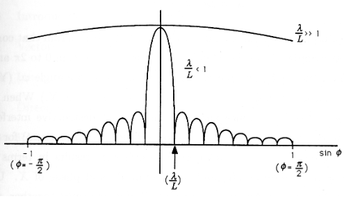
\[|E(φ)|→|\frac {A\sin(\frac {πL} λ \sinφ)} {\frac {πL} λ \sinφ}| \nonumber \]
This function is plotted in theFigure for two values of \(\frac L λ\) the width of the slit measured in wavelengths. When \(\frac L λ<<1\) (i.e., \(/frac λ L >>1\)), then the light is uniformly distributed on the screen. However, when \(\frac L λ>1(\frac λ L<1)\), then the function has many zeros for \(\frac| \sin φ|<1\), as illustrated in the figure. These zeros correspond to dark spots on the screen where the fields radiated from the infinity of points within the slit interfere destructively.
Derive \(|\frac {A\sin(\frac {πL} λ \sinφ)} {\frac {πL} λ \sinφ}|\) from \(|\frac A N \frac {\sin(Nπ\frac d λ \sinφ)} {\sin(π\frac d λ \sinφ)}|\)
(MATLAB) Plot the discrete approximation\
\(∣\frac {\frac A N \sin(Nπ\frac d λ \sinφ)} {\sin(π\frac d λ \sinφ)}∣\)
versus \(\sin φ\) for \(\frac L λ=\frac {Nd} λ=10\) and N=2,4,8,16,32. Compare with the continuous, limiting form
\(∣\frac {A\sin(π\frac L λ \sinφ)} {π\frac L λ \sinφ}∣\)