9.1.3: State Machines

Read this section to go into more detail on FSMs.

---

State machines are a method of modeling systems whose output depends on the entire history of their inputs, and not just on the most recent input. Compared to purely functional systems, in which the output is purely determined by the input, state machines have a performance that is determined by its history. State machines can be used to model a wide variety of systems, including:

• user interfaces, with typed input, mouse clicks, etc.;
• conversations, in which, for example, the meaning of a word "it" depends on the history of things that have been said;
• the state of a spacecraft, including which valves are open and closed, the levels of fuel and oxygen, etc.; and
• the sequential patterns in DNA and what they mean.

State machine models can either be continuous time or discrete time. In continuous time models, we typically assume continuous spaces for the range of values of inputs and outputs, and use differential equations to describe the system's dynamics. This is an interesting and important approach, but it is hard to use it to describe the desired behavior of our robots, for example. The loop of reading sensors, computing, and generating an output is inherently discrete and too slow to be well-modeled as a continuous-time process. Also, our control policies are often highly nonlinear and discontinuous. So, in this class, we will concentrate on discrete-time models, meaning models whose inputs and outputs are determined at specific increments of time, and which are synchronized to those specific time samples. Furthermore, in this chapter, we will make no assumptions about the form of the dependence of the output on the time-history of inputs; it can be an arbitrary function.

Generally speaking, we can think of the job of an embedded system as performing a transduction from a stream (infinite sequence) of input values to a stream of output values. In order to specify the behavior of a system whose output depends on the history of its inputs mathematically, you could think of trying to specify a mapping from i₁, . . . , i_t (sequences of previous inputs) to o_t (current output), but that could become very complicated to specify or execute as the history gets longer. In the state-machine approach, we try to find some set of states of the system, which capture the essential properties of the history of the inputs and are used to determine the current output of the system as well as its next state. It is an interesting and sometimes difficult modeling problem to find a good state-machine model with the right set of states; in this chapter we will explore how the ideas of PCAP can aid us in designing useful models.

One thing that is particularly interesting and important about state machine models is how many ways we can use them. In this class, we will use them in three fairly different ways:

1. Synthetically: State machines can specify a "program" for a robot or other system embedded in the world, with inputs being sensor readings and outputs being control commands.
2. Analytically: State machines can describe the behavior of the combination of a control system and the environment it is controlling; the input is generally a simple command to the entire system, and the output is some simple measure of the state of the system. The goal here is to analyze global properties of the coupled system, like whether it will converge to a steady state, or will oscillate, or will diverge.
3. Predictively: State machines can describe the way the environment works, for example, where I will end up if I drive down some road from some intersection. In this case, the inputs are control commands and the outputs are states of the external world. Such a model can be used to plan trajectories through the space of the external world to reach desirable states, by considering different courses of action and using the model to predict their results.

We will develop a single formalism, and an encoding of that formalism in Python classes, that will serve all three of these purposes.

Our strategy for building very complex state machines will be, abstractly, the same strategy we use to build any kind of complex machine. We will define a set of primitive machines (in this case, an infinite class of primitive machines) and then a collection of combinators that allow us to put primitive machines together to make more complex machines, which can themselves be abstracted and combined to make more complex machines.

Primitive state machines

We can specify a transducer (a process that takes as input a sequence of values which serve as inputs to the state machine, and returns as output the set of outputs of the machine for each input) as a state machine (SM) by specifying:

• a set of states, S,
• a set of inputs, I, also called the input vocabulary,
• a set of outputs, O, also called the output vocabulary,
• a next-state function, n(i_t, s_t) \(\mapsto\) s_t+1, that maps the input at time t and the state at time t to the state at time t + 1,
• an output function, o(i_t, s_t) \(\mapsto\) o_t, that maps the input at time t and the state at time t to the output at time t; and
• an initialstate, s₀, which is the state at time 0.

Here are a few state machines, to give you an idea of the kind of systems we are considering.

• A tick-tock machine that generates the sequence 1, 0, 1, 0, . . . is a finite-state machine that ig­nores its input.
• The controller for a digital watch is a more complicated finite-state machine: it transduces a sequence of inputs (combination of button presses) into a sequence of outputs (combinations of segments illuminated in the display).
• The controller for a bank of elevators in a large office building: it transduces the current set of buttons being pressed and sensors in the elevators (for position, open doors, etc.) into commands to the elevators to move up or down, and open or close their doors.

The very simplest kind of state machine is a pure function: if the machine has no state, and the output function is purely a function of the input, for example, o_t = i_t + 1, then we have an immediate functional relationship between inputs and outputs on the same time step. Another simple class of SMs are finite-state machines, for which the set of possible states is finite. The elevator controller can be thought of as a finite-state machine, if elevators are modeled as being only at one floor or another (or possibly between floors); but if the controller models the exact position of the elevator (for the purpose of stopping smoothly at each floor, for example), then it will be most easily expressed using real numbers for the state (though any real instantiation of it can ultimately only have finite precision). A different, large class of SMs are describable as linear, time-invariant (LTI) systems.

Examples

Let's look at several examples of state machines, with complete formal definitions.

Language acceptor

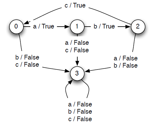
Here is a finite-state machine whose output is true if the input string adheres to a simple pattern, and false otherwise. In this case, the pattern has to be a, b, c, a, b, c, a, b, c, . . ..

It uses the states 0, 1, and 2 to stand for the situations in which it is expecting an a, b, and c, respectively; and it uses state 3 for the situation in which it has seen an input that was not the one that was expected. Once the machine goes to state 3 (sometimes called a rejecting state), it never exits that state.

S = {0, 1, 2, 3}

I = {a, b, c}

O = {true, false}

n(s, i) = \(\begin{cases} 1 & \mathrm{if} \; s=0, i=a\\ 2 & \mathrm{if} \; s=1, i=b\\ 0 & \mathrm{if}\; s=2, i=c\\ 3 & \mathrm{otherwise}\end{cases}\)

o(s, i) = \(\begin{cases}  
\textit{false} \; &\mathrm{if \;} n(s,i) = 3\\
\textit{true} \; &\mathrm{otherwise}
\end{cases}\)

s₀ = 0 

Figure \(\PageIndex{1}\) shows a state transition diagram for this state machine. Each circle represents a state. The arcs connecting the circles represent possible transitions the machine can make; the arcs are labeled with a pair i, o, which means that if the machine is in the state denoted by a circle with label s, and gets an input i, then the arc points to the next state, n(s, i) and the output generated o(s, i) = o. Some arcs have several labels, indicating that there are many different inputs that will cause the same transition. Arcs can only be traversed in the direction of the arrow.

For a state transition diagram to be complete, there must be an arrow emerging from each state for each possible input i (if the next state is the same for some inputs, then we draw the graph more compactly by using a single arrow with multiple labels, as you will see below).

Figure \(\PageIndex{1}\): State transition diagram for language acceptor.

We will use tables like the following one to examine the evolution of a state machine:

time	0	1	2	...
input	i0	i1	i2	...
state	s0	s1	s2	...
output	o1	o2	o3	...

For each column in the table, given the current input value and state we can use the output function o to determine the output in that column; and we use the n function applied to that input and state value to determine the state in the next column. Thus, just knowing the input sequence and s₀, and the next-state and output functions of the machine will allow you to fill in the rest of the table.

For example, here is the state of the machine at the initial time point:

time	0	1	2	...
input	i0			...
state	s0			...
output				...

Using our knowledge of the next state function n, we have:

time	0	1	2	...
input	i0			...
state	s0	s1		...
output				...

and using our knowledge of the output function o, we have at the next input value  

time	0	1	2	...
input	i0	i1		...
state	s0	s1		...
output	o1			...

This completes one cycle of the statement machine, and we can now repeat the process.

Here is a table showing what the language acceptor machine does with input sequence ('a', 'b', 'c', 'a', 'c', 'a', 'b'):

time	0	1	2	3	4	5	6	7
input	'a'	'b'	'c'	'a'	'c'	'a'	'b'
state	0	1	2	0	1	3	3	3
output	True	True	True	True	False	False	False

The output sequence is (True, True, True, True, False, False, False).

Clearly we don't want to analyze a system by considering all input sequences, but this table helps us understand the state transitions of the system model.

To learn more:

Finite-state machine language acceptors can be built for a class of patterns called regular languages. There are many more complex patterns (such as the set of strings with equal numbers of 1's and 0's) that cannot be rec­ognized by finite-state machines, but can be recognized by a specialized kind of infinite-state machine called a stack machine. To learn more about these fundamental ideas in computability theory, start with the Wikipedia article on Computability_theory_(computer_science)

Up and down counter

This machine can count up and down; its state space is the countably infinite set of integers. It starts in state 0. Now, if it gets input u, it goes to state 1; if it gets u again, it goes to state 2. If it gets d, it goes back down to 1, and so on. For this machine, the output is always the same as the next state.

S = integers

I = {u, d}

O = integers

\(n(s,i) = \left\{\begin{matrix} s + 1 \; \; \; \mathrm{if \;} i = u\\ s - 1 \; \; \; \mathrm{if \;} i = d \end{matrix}\right.\)

o(s, i) = n(s, i)

s₀ = 0

Here is a table showing what the up and down counter does with input sequence u, u, u, d, d, u:

time	0	1	2	3	4	5	6
input	u	u	u	d	d	u
state	0	1	2	3	2	1	2
output	1	2	3	2	1	2

The output sequence is 1, 2, 3, 2, 1, 2.

Delay

An even simpler machine just takes the input and passes it through to the output, but with one step of delay, so the kth element of the input sequence will be the k + 1st element of the output sequence. Here is the formal machine definition:

S = anything

I = anything

O = anything

n(s, i) = i

o(s, i) = s

s₀ = 0

Given an input sequence i₀, i₁, i₂, . . ., this machine will produce an output sequence 0, i₀, i₁, i₂, . . .. The initial 0 comes because it has to be able to produce an output before it has even seen an input, and that output is produced based on the initial state, which is 0. This very simple building block will come in handy for us later on.

Here is a table showing what the delay machine does with input sequence 3, 1, 2, 5, 9:

time	0	1	2	3	4	5
input	3	1	2	5	9
state	0	3	1	2	5	9
output	0	3	1	2	5

The output sequence is 0, 3, 1, 2, 5.

Accumulator

Here is a machine whose output is the sum of all the inputs it has ever seen.

S = numbers

I = numbers

O = numbers

n(s, i) = s + i 

o(s, i) = n(s, i)

s₀ = 0

Here is a table showing what the accumulator does with input sequence 100, −3, 4, −123, 10:

time	0	1	2	3	4	5
input	100	-3	4	-123	10
state	0	100	97	101	-22	-12
output	100	97	101	-22	-12

Average2

Here is a machine whose output is the average of the current input and the previous input. It stores its previous input as its state.

S = numbers

I = numbers

O = numbers

n(s, i) = i

o(s, i) = (s + i)/2

s₀ = 0

Here is a table showing what the average2 machine does with input sequence 100, −3, 4, −123, 10:

time	0	1	2	3	4	5
input	100	-3	4	-123	10
state	0	100	-3	4	-123	10
output	50	48.5	0.5	-59.5	-56.5

---

Source: MIT OpenCourseWare, https://ocw.mit.edu/courses/electrical-engineering-and-computer-science/6-01sc-introduction-to-electrical-engineering-and-computer-science-i-spring-2011/unit-1-software-engineering/state-machines/MIT6_01SCS11_chap04.pdf
This work is licensed under a Creative Commons Attribution-NonCommercial-ShareAlike 4.0 License.