3.6: Time Series Methods

Figure \(\PageIndex{1}\): Diagram of trend, cyclical, and seasonal demand patterns.

Time series methods use historical data as the basis of estimating future outcomes. A time series is a series of data points indexed (or listed or graphed) in time order. Most commonly, a time series is a sequence taken at successive equally spaced points in time. Thus, it is a sequence of discrete-time data. Examples of time series are heights of ocean tides, counts of sunspots, and the daily closing value of the Dow Jones Industrial Average.

Time series are very frequently plotted via line charts. Time series are used in statistics, signal processing, pattern recognition, econometrics, mathematical finance, weather forecasting, earthquake prediction, electroencephalography, control engineering, astronomy, communications engineering, and largely in any domain of applied science and engineering which involves temporal measurements.^[4]

In the following, we will elaborate more on some of the simpler time-series methods and go over some numerical examples.

Naïve Method

The simplest forecasting method is the naïve method. In this case, the forecast for the next period is set at the actual demand for the previous period. This method of forecasting may often be used as a benchmark in order to evaluate and compare other forecast methods.

Simple Moving Average

In this method, we take the average of the last “n” periods and use that as the forecast for the next period. The value of “n” can be defined by the management in order to achieve a more accurate forecast. For example, a manager may decide to use the demand values from the last four periods (i.e., n = 4) to calculate the 4-period moving average forecast for the next period.

Example \(\PageIndex{1}\)

Some relevant notation:
D_t = Actual demand observed in period t
F_t = Forecast for period t

Using the following table, calculate the forecast for period 5 based on a 3-period moving average.

Period	Actual Demand
1	42
2	37
3	34
4	40

Solution

Forecast for period 5 = F5 = (D4 + D3 + D2) / 3 = (40 + 34 + 37) / 3 = 111 / 3 = 37

Here is a video explaining simple moving averages.

https://www.linkedin.com/learning/forecasting-using-financial-statements/simple-moving-average

Weighted Moving Average
This method is the same as the simple moving average with the addition of a weight for each one of the last “n” periods. In practice, these weights need to be determined in a way to produce the most accurate forecast. Let’s have a look at the same example, but this time, with weights:

Example \(\PageIndex{2}\)

Period	Actual Demand	Weight
1	42
2	37	0.2
3	34	0.3
4	40	0.5

Solution

Forecast for period 5 = F5 = (0.5 x D4 + 0.3 x D3 + 0.2 x D2) = (0.5 x 40+ 0.3 x 34 + 0.2 x 37) = 37.6

Note that if the sum of all the weights were not equal to 1, this number above had to be divided by the sum of all the weights to get the correct weighted moving average.

Here is a video explaining weighted moving averages.

https://www.linkedin.com/learning/forecasting-using-financial-statements/weighted-moving-average

Exponential Smoothing

This method uses a combination of the last actual demand and the last forecast to produce the forecast for the next period. There are a number of advantages to using this method. It can often result in a more accurate forecast. It is an easy method that enables forecasts to quickly react to new trends or changes. A benefit to exponential smoothing is that it does not require a large amount of historical data. Exponential smoothing requires the use of a smoothing coefficient called Alpha (α). The Alpha that is chosen will determines how quickly the forecast responds to changes in demand. It is also referred to as the Smoothing Factor.

There are two versions of the same formula for calculating the exponential smoothing.

Here is version #1:

F_t = (1 – α) F_t-1 + α D _t-1

Note that α is a coefficient between 0 and 1

For this method to work, we need to have the forecast for the previous period. This forecast is assumed to be obtained using the same exponential smoothing method. If there were no previous period forecast for any of the past periods, we will need to initiate this method of forecasting by making some assumptions. This is explained in the next example.

Example \(\PageIndex{3}\)

Period	Actual Demand	Forecast
1	42
2	37
3	34
4	40
5

Solution

In this example, period 5 is our next period for which we are looking for a forecast. In order to have that, we will need the forecast for the last period (i.e., period 4). But there is no forecast given for period 4. Thus, we will need to calculate the forecast for period 4 first. However, a similar issue exists for period 4, since we do not have the forecast for period 3. So, we need to go back for one more period and calculate the forecast for period 3. As you see, this will take us all the way back to period 1. Because there is no period before period 1, we will need to make some assumption for the forecast of period 1. One common assumption is to use the same demand of period 1 for its forecast. This will give us a forecast to start, and then, we can calculate the forecast for period 2 from there. Let’s see how the calculations work out:

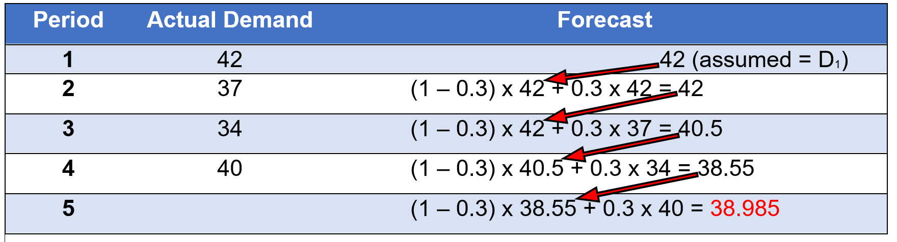
If α = 0.3 (assume it is given here, but in practice, this value needs to be selected properly to produce the most accurate forecast)

Assume F₁ = D₁, which is equal to 42.

Then, calculate F₂ = (1 – α) F₁+ α D₁ = (1 – 0.3) x 42 + 0.3 x 42 = 42

Next, calculate F₃ = (1 – α) F₂+ α D₂ = (1 – 0.3) x 42 + 0.3 x 37 = 40.5

And similarly, F₄ = (1 – α) F₃+ α D₃ = (1 – 0.3) x 40.5 + 0.3 x 34 = 38.55

And finally, F₅ = (1 – α) F₄+ α D₄ = (1 – 0.3) x 38.55 + 0.3 x 40 = 38.985

Figure \(\PageIndex{2}\): Solution for Exponential Smoothing Version 1

Here is a video explaining exponential smoothing using EXCEL.

https://www.linkedin.com/learning/search?keywords=exponential%20smoothing&u=2169170

Here is version #2:

F_t = F_t-1 + α(D_t-1 – F_t-1)

Example \(\PageIndex{4}\)

Assume you are given an alpha of 0.3, F_t-1 = 55

Solution

Figure \(\PageIndex{3}\): Solution for Exponential Smoothing Version 2

Accessible format

Seasonal Index

Many organizations produce goods whose demand is related to the seasons, or changes in weather throughout the year. In these cases, a seasonal index may be used to assist in the calculation of a forecast.

Example \(\PageIndex{5}\)

Season	Previous Sales	Average Sales	Seasonal Index
Winter	390	500	390 / 500 = .78
Spring	460	500	460 / 500 = .92
Summer	600	500	600 / 500 = 1.2
Fall	550	500	550 / 500 = 1.1
Total	2000

Using these calculated indices, we can forecast the demand for next year based on the expected annual demand for the next year. Let’s say a firm has estimated that next year annual demand will be 2500 units.

Solution

Season	Anticipated annual demand	Avg. Sales / Season (2500/4)	Seasonal Factor	New Forecast
Winter		625	0.78	.78 x 625 = 487.5
Spring		625	0.92	.92 x 625 = 575
Summer		625	1.2	1.2 x 625 = 750
Fall		625	1.1	1.1 x 625 = 687.5
	2500