12.4: Interpolation

In many real problems, we do not know the value of a quantity at every possible point. Instead, we collect measurements at a limited number of points. Interpolation is the process of estimating new values inside the range of known data points.

For example, suppose you measure the temperature in a room every hour. If you measured at 11:00 AM and 12:00 PM, but you want to estimate the temperature at 11:30 AM, interpolation is a reasonable approach.

Note

Interpolation vs. Extrapolation

Interpolation estimates values inside the range of your data. Extrapolation estimates values outside the range of your data. Extrapolation is usually riskier because the pattern may not continue beyond the measured data.

 

Example Data: Office Temperature

Assume we measured the temperature in an office from 8:00 AM to 5:00 PM. The time is stored using a 24-hour clock, so 8 means 8:00 AM and 17 means 5:00 PM.

Time	8	9	10	11	12	13	14	15	16	17
Temp (F)	43	58	63	75	80	82	81	77	75	71

 

Linear Interpolation with interp1

The simplest interpolation method is linear interpolation. MATLAB connects each pair of neighboring data points with a straight line and then estimates values along those lines. This is also called piecewise linear interpolation.

 

yNew = interp1(xData, yData, xNew);

 

Here, xData contains the known x-values, yData contains the known y-values, and xNew contains the new x-values where we want estimates.

 

 

Example \(\PageIndex{1}\)

Linear Inrterpolation.

clc; clear; clf;

% Known data points
 timePoints = 8:1:17;
 tempPoints = [43 58 63 75 80 82 81 77 75 71];


% Plot original measurements
plot(timePoints, tempPoints, '-o', 'MarkerFaceColor', 'g')
hold on


% Estimate temperature at 11:30 AM and 2:30 PM
newTimes = [11.5 14.5];
newTemps = interp1(timePoints, tempPoints, newTimes);


% Plot the estimated points
plot(newTimes, newTemps, 'bd')


xlabel('Time of Day')
ylabel('Temperature (F)')
title('Office Temperature: Linear Interpolation')
grid on
axis([8 17 40 90])
hold off

 

Solution

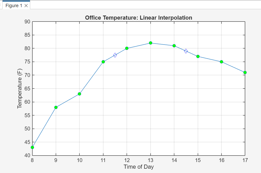
The blue diamond markers show the estimated temperatures at 11:30 AM and 2:30 PM. Because this method uses straight-line sections, the result is easy to understand and often good enough for simple data sets.

 

 

Note

The xData and yData arrays must match. If you have 10 time values, you must also have 10 temperature values.

 

Cubic Spline Interpolation with spline

Linear interpolation is simple, but real data sometimes changes more smoothly than straight-line segments. The spline function uses cubic polynomials to estimate a smooth curve through the data points.

 

yNew = spline(xData, yData, xNew);

 

Cubic spline interpolation is widely used in computer graphics, image processing, animation, and motion planning because it creates smooth transitions between points.

 

Example \(\PageIndex{2}\)

Linear Inrterpolation.

clc; clear; clf;


% Known data points
 timePoints = 8:1:17;
 tempPoints = [43 58 63 75 80 82 81 77 75 71];


% Plot original measurements
plot(timePoints, tempPoints, 'o', 'MarkerFaceColor', 'g')
hold on


% Create many time values to draw a smooth curve
smoothTimes = linspace(8, 17, 50);
smoothTemps = spline(timePoints, tempPoints, smoothTimes);


% Plot spline curve
plot(smoothTimes, smoothTemps, '-r')


% Estimate temperature at selected times
newTimes = [11.5 14.5];
newTemps = spline(timePoints, tempPoints, newTimes);
plot(newTimes, newTemps, 'bd')


xlabel('Time of Day')
ylabel('Temperature (F)')
title('Office Temperature: Cubic Spline Interpolation')
grid on
axis([8 17 40 90])
hold off

 

Solution

The green circle markers represent the known data points.

The red line represents the estimated temperatures for 50 time points between 8:00 AM and 5:00 PM.

The blue diamond markers show the estimated temperatures at 11:30 AM and 2:30 PM.

 

Caution

Common Mistake

Do not assume that a smoother curve is always more accurate. A spline may look nicer, but the accuracy depends on how the real system behaves.