1.3: Charge and Current

As already noted, charge is an attractive force. It is denoted by the letter \(Q\) and has units of coulombs. Electrons are negatively charged and protons are positively charged. All electrons and protons exhibit the same magnitude of charge, roughly 1.602E−19 coulombs. Thus, one coulomb is equivalent to the charge exhibited by approximately 1/1.602E−19, or 6.242E18 electrons. Further, opposite charges attract while like charges repel, similar to the poles of a magnet.

It is possible to move charge from one point to another. The rate of charge movement over time is called current. It is denoted by the letter \(I\) and has units of amps (or amperes)¹. One amp of current is defined as one coulomb per second.

\[1 \text{ amp } \equiv 1 \text{ coulomb } / 1 \text{ second } \label{2.1} \]

That is, one amp can be visualized as approximately 6.242E18 electrons passing through a wire in a period of one second. Consider Figure 2.3.1 .

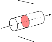
Figure 2.3.1 : Defining current as charge flow through a wire.

Here we have a wire with electrons flowing through it in the direction of the arrow. We cut this wire with an imaginary plane, leaving us with the highlighted disk. Now imagine that we could count the number of electrons passing through this disk over the course of one second. Because we know the charge possessed by one electron, we simply multiply the number of electrons by the charge for each to yield the total charge, and thus we arrive at the current. As a formula:

\[I = Q / t \label{2.2} \]

where

• \(I\) is the current in amps,
• \(Q\) is the the charge in coulombs,
• \(t\) is the time in seconds.

A common analogy for electric current is the flow of water through a pipe or river. Just as we can imagine water flow as “gallons or liters per minute”, we imagine electric current as “coulombs per second”.

Example 2.3.1

In the course of one-half second, a certain battery delivers a charge of three coulombs. Determine the resulting current.

Solution

\[I = \frac{Q}{t} \nonumber \]

\[I = \frac{3C}{0.5s} \nonumber \]

\[I = 6 A \nonumber \]

Example 2.3.2

A device delivers a current of 25 mA. Determine the charge transferred in two seconds along with the equivalent total number of electrons.

Solution

\[I = \frac{Q}{t} \nonumber \]

\[Q = I \times t \nonumber \]

\[Q = 25 mA \times 2s \; \text{ from Definition \ref{2.1}, amp-seconds is coulombs} \nonumber \]

\[Q = 50 mC \nonumber \]

As one coulomb is equivalent to 6.242E18 electrons, just multiply to find the total number of electrons transferred.

\[\text{Total electrons } = Q \times \text{ number of electrons per coulomb } \nonumber \]

\[\text{Total electrons } = 50 mC \times 6.242E18 \nonumber \]

\[\text{Total electrons } = 3.121E17 \text{ electrons} \nonumber \]

In sum, the larger the charge transferred within a given time period, the greater the current. Modern electrical and electronic systems might deal with currents of under a picoamp or, at the other extreme, thousands of amps. That is an astonishing range. It is roughly equivalent to a single drop of water dripping from a leaky faucet each second compared to 1000 times the flow of water over Niagara Falls.

References

¹\(I\) stands for \(I\)ntensity (of current), and was so named by André-Marie Ampère.

Dynamic current

In electrical circuits, the relationship between current and change is governed by calculus, specifically differentiation. Current (I) is the rate of flow of electric charge, and it is defined as the change in charge (Q) with respect to time (t), denoted as I=dQ/dt​. This relationship is based on the fundamental principle that current is the flow of charge over time.

Example: Finding Current when Charge is a Function of Time

Consider a scenario where the charge (Q) on a capacitor is a function of time (t), expressed as Q(t) = 2t² + 3t + 5 coulombs. To find the current (I) at a specific time, we differentiate the charge function with respect to time. By applying the rules of calculus, we find the derivative:

\[ I(t) = \frac{dQ}{dt} = \frac{d}{dt}(2t^2 + 3t + 5) \]

The resulting expression I(t) = 4t + 3 represents the current as a function of time. If you want to find the current at a particular moment, substitute the time value into the equation. For example, to find the current at t=2 seconds:

\[ I(2) = 4×2+3 = 11 Amperes \]

The quantity of charge transferred between two specific time points, t_1​ and t₂​, can be determined by integrating the current function over the given time interval. The integral of the current function I(t) with respect to time over the interval [t_1​ , t₂​] provides the total charge transferred (Q_total​) during that period:

\[ Q_{\text{total}} = \int_{t_1}^{t_2} I(t) \, dt \]

Continue from the above example, we can find the total charge transferred between t1​=1 second and t2​=3 seconds.  

\[ Q_{\text{total}} = \int_{t_1}^{t_2} (4t + 3) \, dt = 22 C \]