3.5.5: Small Signal Models

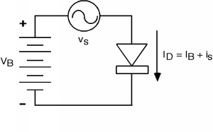
In order to create the linear model, we need to introduce the concept of bias, and large signal and small signal device behavior. Consider the following circuit, shown in Figure \(\PageIndex{1}\). We are applying the sum of two voltages to the diode, \(V_{B}\), the bias voltage (which is assumed to be a DC voltage), and \(v_{s}\), the signal voltage (which is assumed to be AC, or sinusoidal). By definition, we will assume that \(\left| v_{s} \right|\) is much less than \(\left| V_{B} \right|\). As a result of these voltages, there will be a current \(I_{D}\) flowing through the diode. This will consist of two currents: \(I_{B}\), the so-called bias current, and \(i_{s}\), which will be the signal current. Again, we assume that \(i_{s}\) is much smaller than \(I_{B}\).

Figure \(\PageIndex{1}\): Putting together a large signal bias, and a small signal AC excitation

What we would like to do is to see if we can find a linear relationship between \(v_{s}\) and \(i_{s}\), which we could use in our signal analysis. There are two ways we can attack the problem: a graphical approach, and a purely mathematical approach. Let's try the graphical approach first, as it is more intuitive, and then we will confirm what we find out with a mathematical method.

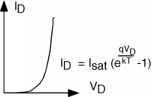
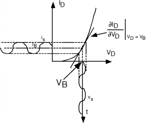
Let's remind ourselves about the \(I \text{-} V\) characteristics of a diode (Figure \(\PageIndex{2}\)). In the present situation, \(V_{D}\) is the sum of two voltages: a DC bias voltage \(V_{B}\) and an AC signal, \(v_{s}\). Let's plot \(V_{D} (t)\) on the \(V_{D}\) axis as shown in Figure \(\PageIndex{3}\).

Figure \(\PageIndex{2}\): Diode \(I \text{-} V\) behavior

Figure \(\PageIndex{3}\): Bias and signal excitation of a diode \(I \text{-} V\) curve

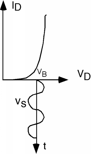
How are we going to figure out what the current is? What we need to do is to project the voltage up onto the characteristic I-V curve, and then project over to the vertical current axis. We do this in Figure \(\PageIndex{4}\).

Figure \(\PageIndex{4}\): Copy and Paste Caption here. (Copyright; author via source)

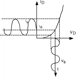
Note that the output current signal is somewhat distorted, which means we do not have linear behavior yet. Let's reduce the amplitude of the signal voltage, as shown in Figure \(\PageIndex{5}\). Now we see two things: a) the output is much less distorted, so we must getting a more linear behavior, and b) we could get the amplitude of the output signal \(i_{s}\) simply by multiplying the input signal \(v_{s}\) by the slope of the I-V curve at the point where the device is biased. We have replaced the non-linear I-V curve of the diode by a linear one, which is applicable over the range of the signal voltage.

\[i_{s} = \left. \frac{\partial}{\partial V_{D}} \left(V_{D}\right) \right| _{I_{D} = I_{B}} \nonumber \]

Figure \(\PageIndex{5}\): With a smaller signal, the response is more linear

To get the slope, we need a few simple equations: \[I_{D} = I_{\text{sat}} \left( e^{\frac{q V_{D}}{kT}} - 1 \right) \simeq I_{\text{sat}} e^{\frac{q V_{D}}{kT}} \nonumber \]

\[ \frac{\partial}{\partial V_{D}} \left(I_{D}\right) = \frac{q}{kT} I_{\text{sat}} e^{\frac{q V_{D}}{kT}} \nonumber \]

When we evaluate the partial derivative at voltage \(V_{D}\), we note that \[I_{\text{sat}} e^{\frac{q V_{D}}{kT}} = I_{B} \nonumber \]

and hence, the slope of the curve is just \(\frac{q}{kT} I_{B}\) or \(40 I_{B}\), since \(\frac{q}{kT}\) just has a value of \(40 \mathrm{~V}^{-1}\) at room temperatures. Note that current divided by voltage is just conductance, (which is just the inverse of resistance) and so we have found the small signal linear conductance for the diode.

As far as the AC signal generator is concerned, we could replace the diode with a resistor whose value is the inverse of the conductance, or \(r = \frac{1}{40} I_{B}\), where \(I_{B}\) is the DC bias current through the diode.

Students are sometimes confused about how we can replace a diode, which only conducts in one direction, with a resistor, which conducts both ways. The answer is to look carefully at Figure \(\PageIndex{5}\). As the AC signal voltage rises and falls, the AC output current also increases and decreases in the same manner. Over the limited range of the AC signal parameters, the diode is indeed a linear signal element, not a rectifying one, as it is for large signal applications.

Now let's get the same answer from a purely mathematical approach. \[I_{D} = I_{B} + i_{s} = I_{\text{sat}} \left( e^{\frac{q V_{D}}{kT}} - 1 \right) \simeq e^{\frac{q \left( V_{B}+v_{s} \right)}{kT}} \nonumber \]

In the last expression, we dropped the \(-1\) as it is very small compared to the exponential term and can be neglected.

Now we note that: \[e^{\frac{q \left( V_{B}+v_{s} \right)}{kT}} = e^{\frac{q V_{B}}{kT}} e^{\frac{q v_{s}}{kT}} \nonumber \]

And, for the second exponential, if \(q V_{B}\) is much less than \(kT\), \[e^{\frac{q V_{s}}{kT}} \simeq 1 + \frac{q v_{s}}{kT} + \ldots \nonumber \]

where we have used the power series expansion for the exponential, but have only taken the first two terms. Thus \[I_{B} + i_{s} \simeq I_{\text{sat}} e^{\frac{q V_{B}}{kT}} \left( 1 + \frac{q v_{s}}{kT} \right) \nonumber \]

Obviously \[I_{B} = I_{\text{sat}} e^{\frac{q V_{B}}{kT}} \nonumber \]

and \[\begin{array}{l} i_{s} &= I_{\text{sat}} e^{\frac{q V_{B}}{kT}} \left( \frac{q}{kT} v_{s} \right) \\ &= \frac{q}{kT} I_{B} v_{s} \end{array} \nonumber \]

which gives us the same result as before: \[\frac{i_{s}}{v_{s}} = \frac{q}{kT} I_{B} \nonumber \]