3.1.3: Quantity of movement equation

Last updated
Save as PDF

Page ID: 78100

\( \newcommand{\vecs}[1]{\overset { \scriptstyle \rightharpoonup} {\mathbf{#1}} } \) \( \newcommand{\vecd}[1]{\overset{-\!-\!\rightharpoonup}{\vphantom{a}\smash {#1}}} \)\(\newcommand{\id}{\mathrm{id}}\) \( \newcommand{\Span}{\mathrm{span}}\) \( \newcommand{\kernel}{\mathrm{null}\,}\) \( \newcommand{\range}{\mathrm{range}\,}\) \( \newcommand{\RealPart}{\mathrm{Re}}\) \( \newcommand{\ImaginaryPart}{\mathrm{Im}}\) \( \newcommand{\Argument}{\mathrm{Arg}}\) \( \newcommand{\norm}[1]{\| #1 \|}\) \( \newcommand{\inner}[2]{\langle #1, #2 \rangle}\) \( \newcommand{\Span}{\mathrm{span}}\) \(\newcommand{\id}{\mathrm{id}}\) \( \newcommand{\Span}{\mathrm{span}}\) \( \newcommand{\kernel}{\mathrm{null}\,}\) \( \newcommand{\range}{\mathrm{range}\,}\) \( \newcommand{\RealPart}{\mathrm{Re}}\) \( \newcommand{\ImaginaryPart}{\mathrm{Im}}\) \( \newcommand{\Argument}{\mathrm{Arg}}\) \( \newcommand{\norm}[1]{\| #1 \|}\) \( \newcommand{\inner}[2]{\langle #1, #2 \rangle}\) \( \newcommand{\Span}{\mathrm{span}}\)\(\newcommand{\AA}{\unicode[.8,0]{x212B}}\)

The quantity of movement equation in a fluid (also referred to as momentum equation) is the second Newton law expression applied to a fluid:

\[\sum \vec{F} = m \dfrac{d(\vec{V})}{dt}.\]

The forces exerted over the matter, solid or fluid, can be of two types:

Distance-exerted, e.g., gravitational, electric, magnetic; related to mass or volume.
Contact-exerted, e..g, pressure or friction, related to the surface of contact.

Euler equation

We assume herein that the fluid is inviscous and, therefore, we do not consider frictional forces. The only sources of forces are pressure and gravity. We consider one-dimensional flow along the longitudinal axis.

截屏2022-01-14 下午8.54.09.png
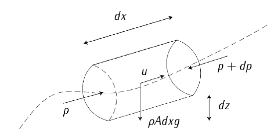
Figure 3.4: Quantity of movement. Adapted from \(F_{\text{RANCHINI}}\) et al. [4].

Assume there is a fluid particle with circular section \(A\) and longitude \(dx\) moving with velocity \(u\) along direction \(x\). Apply second Newton law (\(m \dot{u} = \sum F\); \(m = \rho Adx\)):

\[(\rho A dx) \dfrac{du}{dt} = -Adp - (\rho A dx) g \dfrac{dz}{dx}.\label{eq3.1.3.2}\]

The force due to gravity only affects in the direction of axis \(x\).

Considering a reference frame attached to the particle in which \(dt = \dfrac{dx}{u}\) (stationary flow), the acceleration can be written as \(\tfrac{du}{dt} = \dfrac{du}{dx/u}\) and Equation (\(\ref{eq3.1.3.2}\)), dividing by \(Adx\). yields:

\[\rho u \dfrac{du}{dx} = - \dfrac{dp}{dx} - \rho g \dfrac{dz}{dx}.\label{eq3.1.3.3}\]

Equation (\(\ref{eq3.1.3.3}\)) is referred to as Euler equation. This is the unidimensional case. The Euler equation is more complex, considering the tridimensional motion. The complete equation will be seen is posterior courses of fluid mechanics.

Bernoulli equation

Consider Equation (\(\ref{eq3.1.3.3}\)) and notice that the particle moves on the direction of the streamline. If the flow is incompressible (or there exist a relation between pressure and density, relation called barotropy), the equation can be integrated along the streamline:

\[\rho \dfrac{u^2}{2} + p + \rho gz = C.\label{eq3.1.3.4}\]

The value of the constant of integration, \(C\), should be calculated with the known conditions of a point. Bernouilli equation expresses that the sum of the dynamic pressure (\(\rho \tfrac{u^2}{2}\)), the static pressure (\(p\)), and the piezometric pressure (\(\rho g z\)) is constant along a stream tube.

In the case of the air moving around an airplane, the term \(\rho g z\) does not vary significantly between the different points of the streamline and can be neglected. Equation (\(\ref{eq3.1.3.4}\)) is then simplified to:

\[\rho \dfrac{u^2}{2} + p = C.\]

This does not occur in liquids, where the density is an order of thousands higher than in gases and the piezometric term is always as important as the rest of terms (except if the movement is horizontal).

If at any point of the streamline the velocity is null, the point will be referred to as stagnation point. At that point, the pressure takes a value known as stagnation pressure (\(p_T\)), so that at any other point holds:

\[u = \sqrt{2 \dfrac{p_T - p}{\rho}}.\]