
5.3: Exercises
- Page ID
- 77964

\( \newcommand{\vecs}[1]{\overset { \scriptstyle \rightharpoonup} {\mathbf{#1}} } \)
\( \newcommand{\vecd}[1]{\overset{-\!-\!\rightharpoonup}{\vphantom{a}\smash {#1}}} \)
\( \newcommand{\id}{\mathrm{id}}\) \( \newcommand{\Span}{\mathrm{span}}\)
( \newcommand{\kernel}{\mathrm{null}\,}\) \( \newcommand{\range}{\mathrm{range}\,}\)
\( \newcommand{\RealPart}{\mathrm{Re}}\) \( \newcommand{\ImaginaryPart}{\mathrm{Im}}\)
\( \newcommand{\Argument}{\mathrm{Arg}}\) \( \newcommand{\norm}[1]{\| #1 \|}\)
\( \newcommand{\inner}[2]{\langle #1, #2 \rangle}\)
\( \newcommand{\Span}{\mathrm{span}}\)
\( \newcommand{\id}{\mathrm{id}}\)
\( \newcommand{\Span}{\mathrm{span}}\)
\( \newcommand{\kernel}{\mathrm{null}\,}\)
\( \newcommand{\range}{\mathrm{range}\,}\)
\( \newcommand{\RealPart}{\mathrm{Re}}\)
\( \newcommand{\ImaginaryPart}{\mathrm{Im}}\)
\( \newcommand{\Argument}{\mathrm{Arg}}\)
\( \newcommand{\norm}[1]{\| #1 \|}\)
\( \newcommand{\inner}[2]{\langle #1, #2 \rangle}\)
\( \newcommand{\Span}{\mathrm{span}}\) \( \newcommand{\AA}{\unicode[.8,0]{x212B}}\)
\( \newcommand{\vectorA}[1]{\vec{#1}} % arrow\)
\( \newcommand{\vectorAt}[1]{\vec{\text{#1}}} % arrow\)
\( \newcommand{\vectorB}[1]{\overset { \scriptstyle \rightharpoonup} {\mathbf{#1}} } \)
\( \newcommand{\vectorC}[1]{\textbf{#1}} \)
\( \newcommand{\vectorD}[1]{\overrightarrow{#1}} \)
\( \newcommand{\vectorDt}[1]{\overrightarrow{\text{#1}}} \)
\( \newcommand{\vectE}[1]{\overset{-\!-\!\rightharpoonup}{\vphantom{a}\smash{\mathbf {#1}}}} \)
\( \newcommand{\vecs}[1]{\overset { \scriptstyle \rightharpoonup} {\mathbf{#1}} } \)
\( \newcommand{\vecd}[1]{\overset{-\!-\!\rightharpoonup}{\vphantom{a}\smash {#1}}} \)
\(\newcommand{\avec}{\mathbf a}\) \(\newcommand{\bvec}{\mathbf b}\) \(\newcommand{\cvec}{\mathbf c}\) \(\newcommand{\dvec}{\mathbf d}\) \(\newcommand{\dtil}{\widetilde{\mathbf d}}\) \(\newcommand{\evec}{\mathbf e}\) \(\newcommand{\fvec}{\mathbf f}\) \(\newcommand{\nvec}{\mathbf n}\) \(\newcommand{\pvec}{\mathbf p}\) \(\newcommand{\qvec}{\mathbf q}\) \(\newcommand{\svec}{\mathbf s}\) \(\newcommand{\tvec}{\mathbf t}\) \(\newcommand{\uvec}{\mathbf u}\) \(\newcommand{\vvec}{\mathbf v}\) \(\newcommand{\wvec}{\mathbf w}\) \(\newcommand{\xvec}{\mathbf x}\) \(\newcommand{\yvec}{\mathbf y}\) \(\newcommand{\zvec}{\mathbf z}\) \(\newcommand{\rvec}{\mathbf r}\) \(\newcommand{\mvec}{\mathbf m}\) \(\newcommand{\zerovec}{\mathbf 0}\) \(\newcommand{\onevec}{\mathbf 1}\) \(\newcommand{\real}{\mathbb R}\) \(\newcommand{\twovec}[2]{\left[\begin{array}{r}#1 \\ #2 \end{array}\right]}\) \(\newcommand{\ctwovec}[2]{\left[\begin{array}{c}#1 \\ #2 \end{array}\right]}\) \(\newcommand{\threevec}[3]{\left[\begin{array}{r}#1 \\ #2 \\ #3 \end{array}\right]}\) \(\newcommand{\cthreevec}[3]{\left[\begin{array}{c}#1 \\ #2 \\ #3 \end{array}\right]}\) \(\newcommand{\fourvec}[4]{\left[\begin{array}{r}#1 \\ #2 \\ #3 \\ #4 \end{array}\right]}\) \(\newcommand{\cfourvec}[4]{\left[\begin{array}{c}#1 \\ #2 \\ #3 \\ #4 \end{array}\right]}\) \(\newcommand{\fivevec}[5]{\left[\begin{array}{r}#1 \\ #2 \\ #3 \\ #4 \\ #5 \\ \end{array}\right]}\) \(\newcommand{\cfivevec}[5]{\left[\begin{array}{c}#1 \\ #2 \\ #3 \\ #4 \\ #5 \\ \end{array}\right]}\) \(\newcommand{\mattwo}[4]{\left[\begin{array}{rr}#1 \amp #2 \\ #3 \amp #4 \\ \end{array}\right]}\) \(\newcommand{\laspan}[1]{\text{Span}\{#1\}}\) \(\newcommand{\bcal}{\cal B}\) \(\newcommand{\ccal}{\cal C}\) \(\newcommand{\scal}{\cal S}\) \(\newcommand{\wcal}{\cal W}\) \(\newcommand{\ecal}{\cal E}\) \(\newcommand{\coords}[2]{\left\{#1\right\}_{#2}}\) \(\newcommand{\gray}[1]{\color{gray}{#1}}\) \(\newcommand{\lgray}[1]{\color{lightgray}{#1}}\) \(\newcommand{\rank}{\operatorname{rank}}\) \(\newcommand{\row}{\text{Row}}\) \(\newcommand{\col}{\text{Col}}\) \(\renewcommand{\row}{\text{Row}}\) \(\newcommand{\nul}{\text{Nul}}\) \(\newcommand{\var}{\text{Var}}\) \(\newcommand{\corr}{\text{corr}}\) \(\newcommand{\len}[1]{\left|#1\right|}\) \(\newcommand{\bbar}{\overline{\bvec}}\) \(\newcommand{\bhat}{\widehat{\bvec}}\) \(\newcommand{\bperp}{\bvec^\perp}\) \(\newcommand{\xhat}{\widehat{\xvec}}\) \(\newcommand{\vhat}{\widehat{\vvec}}\) \(\newcommand{\uhat}{\widehat{\uvec}}\) \(\newcommand{\what}{\widehat{\wvec}}\) \(\newcommand{\Sighat}{\widehat{\Sigma}}\) \(\newcommand{\lt}{<}\) \(\newcommand{\gt}{>}\) \(\newcommand{\amp}{&}\) \(\definecolor{fillinmathshade}{gray}{0.9}\)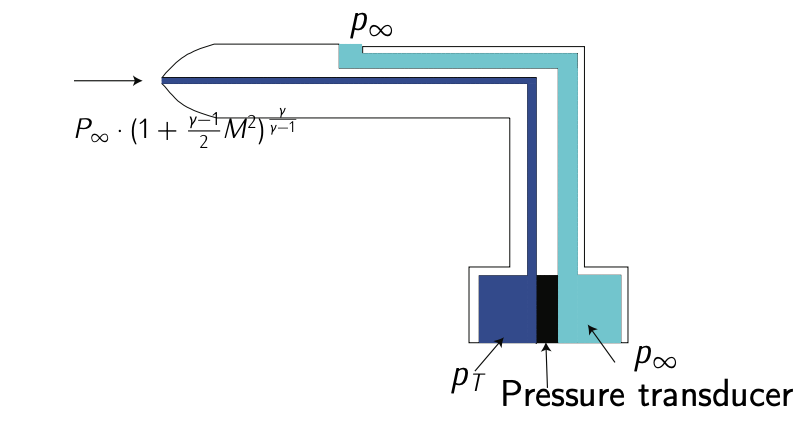
Figure 5.19L Pitot Tube.
Aircraft use pitot tubes to measure airspeed. They consists of a tube pointing directly into the fluid flow, such that the moving fluid is brought to rest (stagnation pressure of the air, \(p_T\)). Typically, pitot tubes include also a static port to measure the static pressure of the air (\(p_{\infty}\)). See Figure 5.19 as illustration considering the air as a compressible flow.
Consider the following measurements on board the aircraft:
- The Pitot tube measures a stagnation pressure \(p_T = 36975\ Pa\).
- The static part measures a static pressure of \(p_{\infty} = 22500\ Pa\).
Assume also that:
- the air can be considered an ideal gas.
- the air should be considered a compressible fluid. For compressible flow, one has that
\[P_T = P_{\infty} \cdot \left (1 + \dfrac{\gamma - 1}{2} M^2 \right )^{\tfrac{\gamma}{\gamma - 1}}, \nonumber \]
with \(\gamma = 1.4\) the adiabatic coefficient of air, and \(M\) the Mach number:
\[M = \sqrt{V_{TAS}}{\sqrt{\gamma RT}} \nonumber \]
Calculate the calibrated airspeed of the aircraft (CAS).8
- Answer
-
Notice that one can apply Bernoulli’s equation to fluid’s stream line within the Pitot tube. Assuming compressible flow, one has:
\[P_T = P_{\infty} \cdot \left (1 + \dfrac{\gamma - 1}{2} M^2 \right )^{\tfrac{\gamma}{\gamma - 1}}. \nonumber \]
Assuming also the air can be considered an ideal gas, one has:
\[P = \rho \cdot R \cdot T. \nonumber \]
In addition, one has the following relation:
\[M = \dfrac{V_{TAS}}{\sqrt{\gamma RT}}. \nonumber \]
All in all, elaborating with this three equations, one has:
\[P_T = P_{\infty} \cdot \left (1 + \dfrac{\gamma - 1}{2} \dfrac{\rho_{\infty} \cdot V_{TAS}^2}{\gamma \cdot P_{\infty}} \right )^{\tfrac{\gamma}{\gamma - 1}}. \nonumber \]
Considering \(P_T - P_{\infty} = \Delta P\) and isolating \(V_{TAS}^2\):
\[V_{TAS}^2 = \dfrac{2\gamma}{\gamma - 1} \cdot \dfrac{P_{\infty}}{\rho_{\infty}} \left (\left (\dfrac{\Delta P}{P_{\infty}} + 1 \right )^{\tfrac{\gamma - 1}{\gamma}} - 1 \right ). \nonumber \]
However, one should notice that only with the pitot tube and the static port, neither temperature nor density can be measured. Thus, \(V_{TAS}\) can not be directly calculated (we would need additional instruments/sensors). This is the reason behind the Calibrated Airspeed (CAS) concept: the true airspeed an aircraft would have if flying with standard mean sea level conditions. Thus, CAS is defined as follows:
\[V_{CAS}^2 = \dfrac{2\gamma}{\gamma - 1} \cdot \dfrac{P_{MSL}}{\rho_{MSL}} \left (\left (\dfrac{\Delta P}{P_{MSL}} + 1 \right )^{\tfrac{\gamma - 1}{\gamma}} - 1 \right ).\label{eq5.3.8} \]
Indeed, the airspeed that is displayed in the cockpit to the pilot (referred to as Indicated Airspeed) is the CAS speed corrected with instrument errors.
Now, entering in Eq. \ref{eq5.3.8} with the values given in the statement, one has the solution to the problem:
\[V_{CAS} = 150\ m/s.\nonumber \]
8. assume mean sea level conditions are the standard ones according to ISA, \(P_{MSL} = 101325\ Pa\) and \(\rho_{MSL} = 1.225\ kg/m^3\)