7.2.1: Fundamental of stability

Last updated
Save as PDF

Page ID: 78158

\( \newcommand{\vecs}[1]{\overset { \scriptstyle \rightharpoonup} {\mathbf{#1}} } \) \( \newcommand{\vecd}[1]{\overset{-\!-\!\rightharpoonup}{\vphantom{a}\smash {#1}}} \)\(\newcommand{\id}{\mathrm{id}}\) \( \newcommand{\Span}{\mathrm{span}}\) \( \newcommand{\kernel}{\mathrm{null}\,}\) \( \newcommand{\range}{\mathrm{range}\,}\) \( \newcommand{\RealPart}{\mathrm{Re}}\) \( \newcommand{\ImaginaryPart}{\mathrm{Im}}\) \( \newcommand{\Argument}{\mathrm{Arg}}\) \( \newcommand{\norm}[1]{\| #1 \|}\) \( \newcommand{\inner}[2]{\langle #1, #2 \rangle}\) \( \newcommand{\Span}{\mathrm{span}}\) \(\newcommand{\id}{\mathrm{id}}\) \( \newcommand{\Span}{\mathrm{span}}\) \( \newcommand{\kernel}{\mathrm{null}\,}\) \( \newcommand{\range}{\mathrm{range}\,}\) \( \newcommand{\RealPart}{\mathrm{Re}}\) \( \newcommand{\ImaginaryPart}{\mathrm{Im}}\) \( \newcommand{\Argument}{\mathrm{Arg}}\) \( \newcommand{\norm}[1]{\| #1 \|}\) \( \newcommand{\inner}[2]{\langle #1, #2 \rangle}\) \( \newcommand{\Span}{\mathrm{span}}\)\(\newcommand{\AA}{\unicode[.8,0]{x212B}}\)

A vehicle is said to be in equilibrium when remains constant or the movement is uniform, that is, both the linear and angular quantity of movement are constant. In the case of an aircraft, the state of equilibrium typically refers to an uniform movement in which the angular velocities are null, and then the movement is simply a translation.

The stability is a property related with the state of equilibrium, which studies the behavior of the aircraft when any of the variables describing its state of equilibrium suffers from a variation (for instance a wind gust). The variation in one of those variables is typically referred to as perturbation.

The stability can be studied in two different ways depending on the time scale:

Static stability.
Dynamic stability.

Static stability

The interest lies on the instant of time immediately after the perturbation takes place. In the static stability, the forces and torques which appear immediately after the perturbation are studied. If the value of the state variables describing the equilibrium tends to increase or amplify, the state of equilibrium is statically unstable. On the contrary, it is statically stable. Figure 7.10 shows a sketch of an aircraft with three different options for the static stability after a pitch down disturbance, e.g., a downwards wind gust.

Dynamic stability

截屏2022-02-07 下午9.42.32.png
Figure 7.11: Diagram showing the three main cases for aircraft pitch dynamic stability. Here all three cases are for a statically stable aircraft. Following a pitch disturbance, three cases are shown: Aircraft is dynamically unstable (although statically stable); Aircraft is dynamically damped (and statically stable); Aircraft is dynamically overdamped (and statically stable). © User:Ariadacapo / Wikimedia Commons / CC0-1.0.

The dynamic stability studies the evolution with time of the different variables of flight (yaw, pitch, and roll angles, velocity, angular velocities, altitude, etc.) when the condition of equilibrium is perturbed. Figure 7.11 shows a sketch of an aircraft with different dynamic-stability behaviors after a pitch down disturbance, e.g., a downwards wind gust. In order to study this evolution we need to solve the system of equation describing the 6DOF movement of the aircraft. As illustrated in Appendix A, the equations are:

\[\vec{F} = m \dfrac{d\vec{V}}{dt},\]

\[\vec{G} = l \dfrac{d\vec{\omega}}{dt}.\]

An aircraft is said to be dynamically stable when after a perturbation the variables describing the movement of the aircraft tend to a stationary value (either the same point of equilibrium or a new one). On the contrary, if the aircraft does not reach an equilibrium it is said to be dynamically unstable.

截屏2022-02-07 下午9.49.03.png
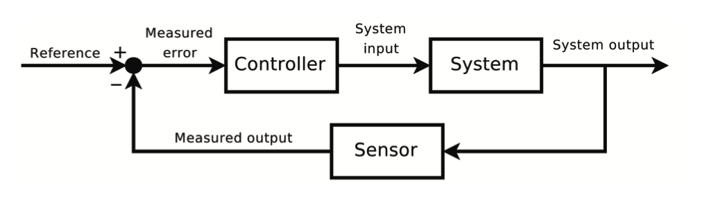
Figure 7.12: Feedback loop to control the dynamic behavior of the system: The sensed value is subtracted from the desired value to create the error signal, which is amplified by the controller. © User:Myself / Wikimedia Commons / CC-BY-SA-3.0.

As the reader might imagine, aircraft are designed to be dynamically stable. Indeed, advanced flight mechanics studies (out of the scope of this book) will focus on the analysis of aircraft stability and control. A typical analysis would consist in: the linearization of the 6DoF equations (for which one needs the so-called stability derivatives); the characterization of the flight modes (for which one would uncouple longitudinal and lateral dynamics and calculate eigenvalues and eigenvectors), i.e., short period, phugoid, spiral, rolling convergence and Dutch roll; the analysis of open loop response (uncontrolled aircraft motion subject to a control actions -a perturbation-, e.g., a throttle step), which would end up activation some of the flight modes; and finally the closed-loop control response (controlled motion of the aircraft), which consists in the fundamentals of an autopliot design (one sets a reference value to track and the control system is designed to correct measured/estimated deviations from it). The reader is referred to Etkin and Reid [2] for a thorough course on this matter.