
9.5: Exercises
- Page ID
- 78371

\( \newcommand{\vecs}[1]{\overset { \scriptstyle \rightharpoonup} {\mathbf{#1}} } \)
\( \newcommand{\vecd}[1]{\overset{-\!-\!\rightharpoonup}{\vphantom{a}\smash {#1}}} \)
\( \newcommand{\dsum}{\displaystyle\sum\limits} \)
\( \newcommand{\dint}{\displaystyle\int\limits} \)
\( \newcommand{\dlim}{\displaystyle\lim\limits} \)
\( \newcommand{\id}{\mathrm{id}}\) \( \newcommand{\Span}{\mathrm{span}}\)
( \newcommand{\kernel}{\mathrm{null}\,}\) \( \newcommand{\range}{\mathrm{range}\,}\)
\( \newcommand{\RealPart}{\mathrm{Re}}\) \( \newcommand{\ImaginaryPart}{\mathrm{Im}}\)
\( \newcommand{\Argument}{\mathrm{Arg}}\) \( \newcommand{\norm}[1]{\| #1 \|}\)
\( \newcommand{\inner}[2]{\langle #1, #2 \rangle}\)
\( \newcommand{\Span}{\mathrm{span}}\)
\( \newcommand{\id}{\mathrm{id}}\)
\( \newcommand{\Span}{\mathrm{span}}\)
\( \newcommand{\kernel}{\mathrm{null}\,}\)
\( \newcommand{\range}{\mathrm{range}\,}\)
\( \newcommand{\RealPart}{\mathrm{Re}}\)
\( \newcommand{\ImaginaryPart}{\mathrm{Im}}\)
\( \newcommand{\Argument}{\mathrm{Arg}}\)
\( \newcommand{\norm}[1]{\| #1 \|}\)
\( \newcommand{\inner}[2]{\langle #1, #2 \rangle}\)
\( \newcommand{\Span}{\mathrm{span}}\) \( \newcommand{\AA}{\unicode[.8,0]{x212B}}\)
\( \newcommand{\vectorA}[1]{\vec{#1}} % arrow\)
\( \newcommand{\vectorAt}[1]{\vec{\text{#1}}} % arrow\)
\( \newcommand{\vectorB}[1]{\overset { \scriptstyle \rightharpoonup} {\mathbf{#1}} } \)
\( \newcommand{\vectorC}[1]{\textbf{#1}} \)
\( \newcommand{\vectorD}[1]{\overrightarrow{#1}} \)
\( \newcommand{\vectorDt}[1]{\overrightarrow{\text{#1}}} \)
\( \newcommand{\vectE}[1]{\overset{-\!-\!\rightharpoonup}{\vphantom{a}\smash{\mathbf {#1}}}} \)
\( \newcommand{\vecs}[1]{\overset { \scriptstyle \rightharpoonup} {\mathbf{#1}} } \)
\(\newcommand{\longvect}{\overrightarrow}\)
\( \newcommand{\vecd}[1]{\overset{-\!-\!\rightharpoonup}{\vphantom{a}\smash {#1}}} \)
\(\newcommand{\avec}{\mathbf a}\) \(\newcommand{\bvec}{\mathbf b}\) \(\newcommand{\cvec}{\mathbf c}\) \(\newcommand{\dvec}{\mathbf d}\) \(\newcommand{\dtil}{\widetilde{\mathbf d}}\) \(\newcommand{\evec}{\mathbf e}\) \(\newcommand{\fvec}{\mathbf f}\) \(\newcommand{\nvec}{\mathbf n}\) \(\newcommand{\pvec}{\mathbf p}\) \(\newcommand{\qvec}{\mathbf q}\) \(\newcommand{\svec}{\mathbf s}\) \(\newcommand{\tvec}{\mathbf t}\) \(\newcommand{\uvec}{\mathbf u}\) \(\newcommand{\vvec}{\mathbf v}\) \(\newcommand{\wvec}{\mathbf w}\) \(\newcommand{\xvec}{\mathbf x}\) \(\newcommand{\yvec}{\mathbf y}\) \(\newcommand{\zvec}{\mathbf z}\) \(\newcommand{\rvec}{\mathbf r}\) \(\newcommand{\mvec}{\mathbf m}\) \(\newcommand{\zerovec}{\mathbf 0}\) \(\newcommand{\onevec}{\mathbf 1}\) \(\newcommand{\real}{\mathbb R}\) \(\newcommand{\twovec}[2]{\left[\begin{array}{r}#1 \\ #2 \end{array}\right]}\) \(\newcommand{\ctwovec}[2]{\left[\begin{array}{c}#1 \\ #2 \end{array}\right]}\) \(\newcommand{\threevec}[3]{\left[\begin{array}{r}#1 \\ #2 \\ #3 \end{array}\right]}\) \(\newcommand{\cthreevec}[3]{\left[\begin{array}{c}#1 \\ #2 \\ #3 \end{array}\right]}\) \(\newcommand{\fourvec}[4]{\left[\begin{array}{r}#1 \\ #2 \\ #3 \\ #4 \end{array}\right]}\) \(\newcommand{\cfourvec}[4]{\left[\begin{array}{c}#1 \\ #2 \\ #3 \\ #4 \end{array}\right]}\) \(\newcommand{\fivevec}[5]{\left[\begin{array}{r}#1 \\ #2 \\ #3 \\ #4 \\ #5 \\ \end{array}\right]}\) \(\newcommand{\cfivevec}[5]{\left[\begin{array}{c}#1 \\ #2 \\ #3 \\ #4 \\ #5 \\ \end{array}\right]}\) \(\newcommand{\mattwo}[4]{\left[\begin{array}{rr}#1 \amp #2 \\ #3 \amp #4 \\ \end{array}\right]}\) \(\newcommand{\laspan}[1]{\text{Span}\{#1\}}\) \(\newcommand{\bcal}{\cal B}\) \(\newcommand{\ccal}{\cal C}\) \(\newcommand{\scal}{\cal S}\) \(\newcommand{\wcal}{\cal W}\) \(\newcommand{\ecal}{\cal E}\) \(\newcommand{\coords}[2]{\left\{#1\right\}_{#2}}\) \(\newcommand{\gray}[1]{\color{gray}{#1}}\) \(\newcommand{\lgray}[1]{\color{lightgray}{#1}}\) \(\newcommand{\rank}{\operatorname{rank}}\) \(\newcommand{\row}{\text{Row}}\) \(\newcommand{\col}{\text{Col}}\) \(\renewcommand{\row}{\text{Row}}\) \(\newcommand{\nul}{\text{Nul}}\) \(\newcommand{\var}{\text{Var}}\) \(\newcommand{\corr}{\text{corr}}\) \(\newcommand{\len}[1]{\left|#1\right|}\) \(\newcommand{\bbar}{\overline{\bvec}}\) \(\newcommand{\bhat}{\widehat{\bvec}}\) \(\newcommand{\bperp}{\bvec^\perp}\) \(\newcommand{\xhat}{\widehat{\xvec}}\) \(\newcommand{\vhat}{\widehat{\vvec}}\) \(\newcommand{\uhat}{\widehat{\uvec}}\) \(\newcommand{\what}{\widehat{\wvec}}\) \(\newcommand{\Sighat}{\widehat{\Sigma}}\) \(\newcommand{\lt}{<}\) \(\newcommand{\gt}{>}\) \(\newcommand{\amp}{&}\) \(\definecolor{fillinmathshade}{gray}{0.9}\)The exercise is related to Master planning for airports. Students will team up in groups of four people each. The exercise is to be completed during the class. Students are allowed to use any mean, e.g., books, laptops, internet, to find a solution to the problem.
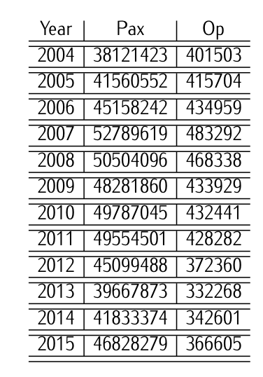
Table 9.7: Historical data [2004-2015 period] about number of passenger and number of operations in the Adolfo-Suarez Madrid Barajas airport.
The historical data contained in Table 9.7 with the number of passengers and the number of operations in the Adolfo-Suarez Madrid Barajas airport for the period 2004-2015 is made available.
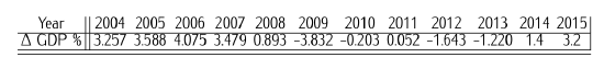
Table 9.8: Historical data [2004-2015 period] of GDP growth.
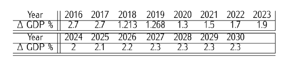
Table 9.9: Forecast [2016-2030] of GDP growth.
Historical data [period 2004-2015] of the Spanish Gross Domestic Product (GDP) [in nominal terms, i.e., not considering inflation] are given in Table 9.8. Also, forecasts 2016-2030 for the World GDP forecast [in nominal terms] from both IMF (International Monetary Found) and CEPREDE7 are given in Table 9.9.
- With these data (Pax and GDP), do a traffic forecast (number of pax. 2016-2030) using econometric models. Find a solution (traffic forecast) for three different scenarios (pessimistic, nominal, optimistic). Depict a sketch figure of the evolution of the number of passenger in the period 2016-2030 for the three scenarios.
The maximum capacity of the Airport Adolfo-Suarez Madrid Barajas has been declared to be 70 Million passenger a year.
- According to the different forecasts, when is it estimated the airport to be non capable of coping with the passengers’ demand?
- What other metrics should we look at (besides that of total amount of passengers) in order to analyze the capacity of the airport? Why?
- Answer
-
Econometric models represent one of the most sophisticated and complex technique in airport demand forecasting. Simple and multiple regression analysis techniques (linear and nonlinear) are often applied.
Multiple regression analysis can be regarded as an extension of simple linear regression analysis (which involves only one independent variable) to the situation where two or more independent variables are considered. The general form of a polynomial regression model for m independent variables is
\[Y = \beta_0 + \beta_1 X_1+ \beta_2 X_2 + ... + \beta_m X_m + \varepsilon, \nonumber \]
where \(\beta_0, \beta_1, ..., \beta_m\) are the regression coefficients that need to be estimated. The independent variables \(X_1, X_2,... , X_m\) may all be separate basic variables, or some of them may be functions of a few basic variables. \(Y\) represents an individual observation and \(\varepsilon\) is the error component reflecting the difference between an individual’s observed response \(Y\) and the true average response \(\mu_{Y|X_1,X_2,...,X_m}\).
In this particular case, for the sake of simplicity, we run a linear regression analysis as follows:
\[Y = \beta_0 + \beta_1 X_1 + \varepsilon, \nonumber \]
where \(Y\) represents individual observations, i.e., values of traffic demand (pax) between years 2004-2015; and \(X_1\) represents the explanatory variables, i.e., the gross domestic product growth in the same period. Therefore, we want to estimate the coefficients \(\beta_0\) and \(\beta_1\) that best fit the data; in other words, we want to estimate the line that minimizes the errors \(\varepsilon\) of the observations. We will use minimum squares method.
Taking years 2004-2015, the solution is:
\[Y = -0.1307 + 2.7182 X,\label{eq9.5.3} \]
Figure 9.17: Linear regression analysis.where \(Y\) represent de % of passenger growth and X represents the percentage of GDP growth. See Figure 9.17. The goodness of fit measured in term of R2 (coefficient of determination) is rather low (0.6080), meaning that the curve does not fit very well the data (as it can be observed from the graph). Other regression might be done in which some observations could be considered outliers or even considering nonlinear functions.
Given Eq. \ref{eq9.5.3}, we build three different scenarios for GDP growth: nominal (the given one in Table 9.8), optimistic (in this case the one in Table 9.8 + 0.5%), and pessimistic (in this case the one in Table 9.8 - 0.5%). Again, notice that other scenarios could have been built yielding different results.
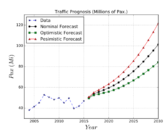
Figure 9.18: Scenarios of traffic forecast.2. When is it estimated the airport to be non capable of coping with the passengers’ demand?
- Pessimistic: 70M Pax exceeded in 2026.
- Nominal: 70M Pax exceeded in 2023.
- Optimistic: 70M Pax exceeded in 2021.
3. What other metrics should we look at (besides that of total amount of passengers) in order to analyze the capacity of the airport? Why?
One should also look at the operations/design hour; Pax/design hour. Also, number of vehicles accessing the airport; number of people using the subway; etc.
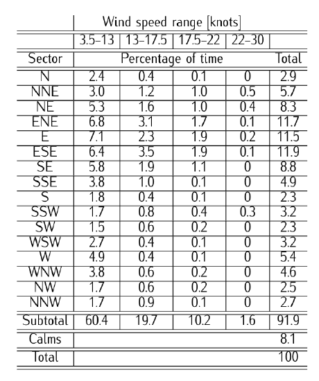
Table 9.10: Example of historical wind data.
For a given site located in Somewhere, historical wind data have been already collected for the last 15 years as illustrated in Table 9.10.
1. Fill in the wind rose diagram sketched bellow and propose the most suitable direction (or directions) for a new runway (or runways).
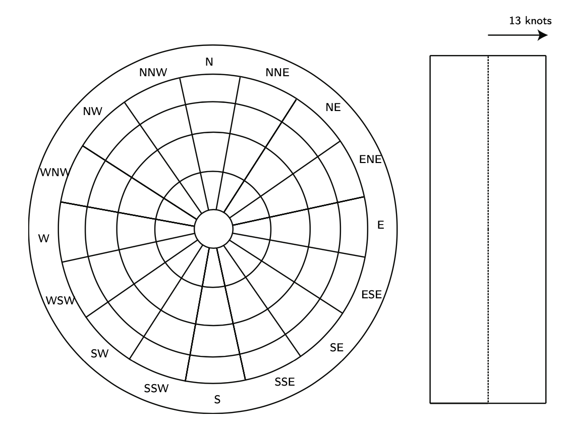
Figure 9.19: Wind Rose coordinate system and template with cross wind component limits of 13 knots.
- Answer
-
According to ICAO’s Annex 14 (Recommendation 3.1):
The number and orientation of runways at an aerodrome should be such that the usability factor of the aerodrome is not less than 95 per cent for the airplanes that the aerodrome is intended to serve.
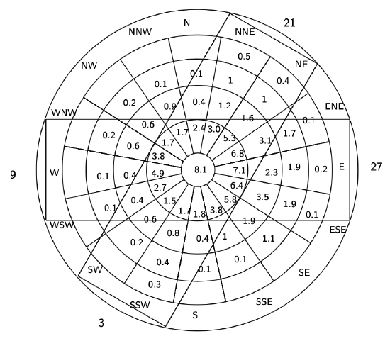
Figure 9.20: Wind coverage for runways 9-27 and 3-21.Then, taking that recommendation into consideration, we first calculate the runway orientation the yields the maximum percentage of wind between parallel lines. This is the runway 9-27 (see Figure 9.20). It will permit around 90-91% of the operations. If one wants to follow the recommendations, we must build another runway. We do that trying to maximize the % of operations. The solution is the 3-21 runway (see Figure 9.20), which would permit around 97.5% of the operations.
The exercise is related to identifying the main aerodrome data for a particular airport. For the airport Adolfo Suarez Madrid Barajas, identify:
1. The following data about the site:
- Aerodrome’s Reference Point;
- Aerodrome’s Elevation;
- Coordinates of the runway’s thresholds;
- Coordinates of the parking positions;
- Mean elevation of each of the thresholds;
- Elevation of the runway’s heads;
- Maximum elevation of the touchdown zone;
- Answer
-
All data can be consulted at AENA’s AIS Adolfo Suarez Madrid Barajas. In particular, one should consult:
- Aerodrome data
- Aerodrome chart
- Aerodrome ground movement chart
- Aircraft parking/docking chart
- Aerodrome obstacle chart
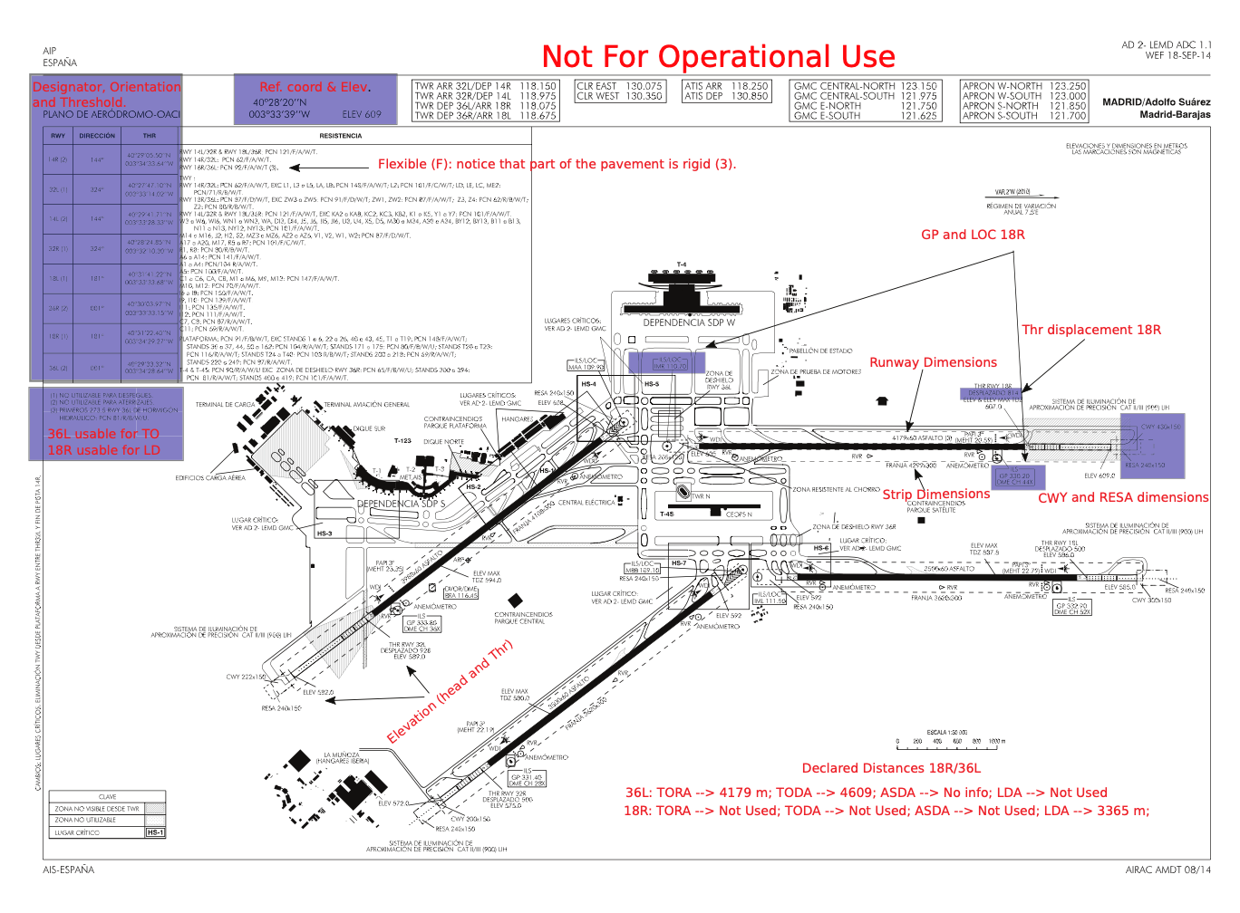
Figure 9.21: Aerodrome data.The solution is sketched in Figure 9.21. Please, notice that the solution to Exercise 9.4 is also given in this Figure.
The exercise is related to identifying the main aerodrome data for a particular airport. For the airport Adolfo Suarez Madrid Barajas (For the runway 36L/14R), identify the following data about the movement area:
- Dimensions (length and width);
- Usability of both 36L and 18R for take-offs and landings.
- Safety areas (strip and runway end safety areas for 36L/18R);
- Displacement of the threshold for 36L and 18R;
- Declared distances for 36L and 18R;
- Identify the localizer and the glide path for the ILS of the runway 18R. Write down their frequencies.
- Pavement Classification Number of runways 36L and 18R. What kind of pavement is it? How can we know it?
All this information can be consulted at Adolfo Suarez Madrid Barajas Aerodrome’s chart given in the appendix.
- Answer
-
All data can be consulted at AENA’s AIS Adolfo Suarez Madrid Barajas consulting the same documents as in Exercise 1.3. The solution is sketched in Figure 9.21.
A regional airport to be designed has the following emplacement characteristics:
- Located at sea level;
- Emplaced in flat terrain;
- Located in a standard latitude of 40 deg (\(\Delta T = 0\)).
The critical aircraft has the following characteristics:
- Reference Field length \(\to\0 1100 m.
- Wingspan \(\to\) 28 m.
Do a preliminary design of the runway according to ICAO’s regulations in App. 14. Follow the following steps (use sketches if needed):
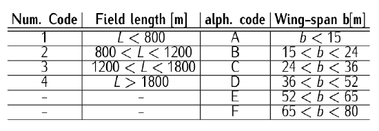
Table 9.11: Runway ICAO categories (alph. code refers to the type of aircraft).
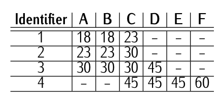
Table 9.12: Minimum runway’s width [m] ICAO identifiers.
- Identify the reference code of the aerodrome (see Table 9.11);
- Select length and width of the runway (see Table 9.12);
- Dimension the safety areas (strip and runway end safety area);
- Identify the designators of the two runway heads according to the runway direction selected in the previous exercise.
- Choose one of the runway’s heads and displace the threshold 100 m. Publish the declared distances of this runway head (notice that the stopway and the clearway need to be considered; if needed dimension them following ICAO recommendations).
The needed information can be found in the tables below and in the appendix containing ICAO’s appendix 14 (3.10-3.17).
- Answer
-
Figure 9.22: Runway design.- The reference code of the aerodrome would be 2C.
- Given that the altitude of the aerodrome is 0, conditions are ISA standard, and there is no slope, the distance should be the given reference field of the critical aircraft (1100 m). Any larger runway would also work but implies over-investment. Width should also be the minimum (30 m) for the same reason.
- Dimension must be at least: Strip (1220 m \(\times\) 180 m) and RESA (60 m \(\times\) 90 m) starting at the edge of the runway head. Authorities recommend RESA length of 120 m for instrumental aerodrome.
- The designators would be 05 and 23.
- There must be a Clearway (length less than have of the take-off run \(\times\) 75 m width from the center line); Stopway is not mandatory, but it must have same width as the runway. Please check Figure 9.22 for the solution.
- Declared distances can be also checked in Figure 9.22. Notice that in case of a SWY, the length of the runway should be 1100 + SWY. ASDA would then be 1100 + SWY.
The exercise is related to identifying the main aerodrome visual aids for a particular airport. For the airport Adolfo Suarez Madrid Barajas, identify:
- the main markings of any of the runways, i.e.:
\(\bullet\) Designator
\(\bullet\) Threshold and pre-threshold
\(\bullet\) Center lines and side line
\(\bullet\) Aiming point
\(\bullet\) Touchdown zone - the main lights of any of the runways.
- the instrumental aids in the airfield, i.e, VOR, DME, ILS. Write down the location and the frequency.
- the main markings in the taxiways.
- the main markings in apron and ramp.
- Answer
-
All data can be consulted at AENA’s AIS Adolfo Suarez Madrid Barajas. In particular, you should consult:
- Aerodrome data
- Aerodrome chart
- Aerodrome ground movement chart
- Aircraft parking/docking chart
The exercise is a continuation of Exercise 9.5.5 , thus related to a preliminary runway design. Assume you have done a preliminary design of the runway, including dimensions, safety areas, etc. (i.e., assume you have assessed Exercise 9.5.5 ). Do a preliminary design of the main markings of the runway, i.e.:
- Designator
- Threshold and pre-threshold
- Center lines and side line
- Aiming point
- Touchdown zone
and the main lights of the runway.
- Answer
-
All data can be consulted at ICAO’s Annex 14 and ICAO’s Runway design manual (Part I and IV).
We want to estimate the take-off distance of a typical commercial jet aircraft. Such aircraft mounts two turbojets, which thrust can be estimated as: \(T = T_0 (1 − k \cdot V^2)\), where \(T\) is the thrust, \(T_0\) is the nominal thrust, \(k\) is a constant and \(V\) is the true airspeed.
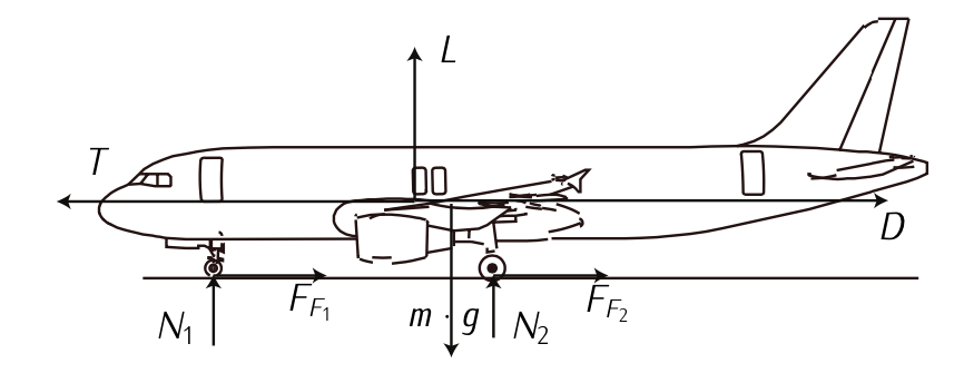
Figure 9.23: Forces during taking off run.
Consider Figure 9.23, where \(g\) is the force due to gravity, \(m\) is the mass of the aircraft, \(F_F\) corresponds to the friction force (being \(\mu_r\) the friction coefficient of the pavement), and \(L\) and \(D\) are lift and drag force, respectively, which can be expressed as:
\[L = C_L \dfrac{1}{2} \rho SV^2; \nonumber \]
\[D = C_D \dfrac{1}{2} \rho SV^2; \nonumber \]
where \(\rho\) is the density of air, \(S\) is the wet surface area of the aircraft, \(C_D\) is the coefficient of drag (which can be approximated to the parasite coefficient of drag, i.e., \(C_D = C_{D_0}\)) and \(C_L\) is the coefficient of lift.8
Find:
- An analytic expression for the take-off distance of this generic aircraft.
Consider a B-737-800, which values can be approximated to:
- \(T_0 = 149000\ [N]\) and \(k = 1 \cdot 10^{-5}\).
- \(C_{D_0} = 0.0357\) (with flap configuration for take-off)
- \(S = 124.65\ [m^2]\);
- \(m = 78300\ [kg] (MTOW)\);
- \(V_{TO} = 1.2 V_{Stall}\) (with flop configuration for take-off). We can consider \(V_{LOF} = 1.1 V_{Stall}\);
- \(V_{stall} = \sqrt{\tfrac{2mg}{\rho S C_{L_{\max}}}}\);
- \(C_{L_{\max}} = 2\) and \(C_L = 0.8 C_{L_{\max}}\).
Moreover, we can consider \(\mu_r = 0.025\).
According to the previously selected numbers:
2. Take-off distance for different altitudes (sea level, 2000 ft, 4000 ft, 6000 ft, 8000 ft, 10000 ft) under calm conditions and maximum take-off weight. Compare these results with the figures published in the 737 Airplane Characteristics for Airport Planning document. Discuss them.
- Answer
-
[1] We apply the 2nd Newton's Law:
\[\sum F_z = 0;\label{eq9.5.6} \]
\[\sum F_x = m \dot{V}.\label{eq9.5.7} \]
Regarding Equation \ref{eq9.5.6}, notice that while rolling on the ground, the aircraft is assumed to be under equilibrium along the vertical axis.
Looking at Figure 9.23, Equations \ref{eq9.5.6}-\ref{eq9.5.7} become:
\[L + N - mg = 0;\label{eq9.5.8} \]
\[T - D - F_F = m \dot{V}.\label{eq9.5.9} \]
being \(L\) the lift, \(N\) the normal force, mg the weight; \(T\) the trust, \(D\) the drag and \(F_F\) the total friction force.
It is well known that:
\[L = C_L \dfrac{1}{2} \rho S V^2;\label{eq9.5.10} \]
\[D = C_D \dfrac{1}{2} \rho SV^2.\label{eq9.5.11} \]
It is also well known that:
\[F_F = \mu_r N. \nonumber \]
Equation \ref{eq9.5.8} state that: \(N = mg - L\). Therefore:
\[F_F = \mu_r (mg - L).\label{eq9.5.13} \]
Given that \(T = T_0 (1 - kV^2)\), with Equation \ref{eq9.5.13} and Equations \ref{eq9.5.10}-\ref{eq9.5.11}. Equation \ref{eq9.5.9} becomes:
\[(\dfrac{T_0}{m} - \mu_r g) + \dfrac{(\rho S(\mu_r - C_D) - 2T_0 k)}{2m}V^2 = \dot{V}.\label{eq9.5.14} \]
Now, we have to integrate Equation \ref{eq9.5.14}.
In order to do so, we know, as it was stated in the statement, that: \(T_0, m, \mu_r, g, \rho, S, C_L, C_D\) and \(k\) can be considered constant along the take off phase.
We have that:
\[\dfrac{dV}{dt} = \dfrac{dV}{dx} \dfrac{dx}{dt}, \nonumber \]
and knowing that \(\tfrac{dx}{dt} = V\), Equation \ref{eq9.5.14} becomes:
\[\dfrac{(\tfrac{T_0}{m} - \mu_r g) + \tfrac{(\rho S (\mu_r C_L - C_D) - 2T_0k)}{2m} V^2}{V} = \dfrac{dV}{dx}.\label{eq9.5.16}\)
In order the simplify Equation \ref{eq9.5.16}:
- \((\tfrac{T_0}{m} - \mu_r g) = A\);
- \(\tfrac{(\rho S(\mu_r C_L - C_D) - 2 T_0k)}{2m} = B\).
We proceed on integrating Equation \ref{eq9.5.16} between \(x = 0\) and \(x_{LOF}\) (the distance of lift off); \(V = 0\) (assuming the maneuver starts with the aircraft at rest) and the lift off speed: \(V_{LOF}\). It holds that:
\[\int_{0}^{x_{LOF}} dx = \int_{0}^{V_{LOF}} \dfrac{VdV}{A + BV^2}. \nonumber \]
Intergrating:
\[\langle x \rangle_0^{x_{LOF}} = \langle \dfrac{1}{2B} Ln (A + BV^2) \rangle_0^{V_{LOF}} \nonumber \]
Substituting the upper and lower limits:
\[x_{LOF} = \dfrac{1}{2B} Ln (1 + \dfrac{B}{A} V_{LOF}^2).\label{eq9.5.19} \]
[2] With the values given in the statement and using Eq \ref{eq9.5.19} and substituting it yields:
- \(x_{LOF} (h = 0) = 2605.5\ [m]\)
- \(x_{LOF} (h = 2000\ ft) = 2764.4\ [m]\)
- \(x_{LOF} (h = 4000\ ft) = 2935.4\ [m]\)
- \(x_{LOF} (h = 6000\ ft) = 3119.7\ [m]\)
- \(x_{LOF} (h = 8000\ ft) = 33186\ [m]\)
- \(x_{LOF} (h = 10000\ ft) = 3533.4\ [m]\)
Figure 9.24 illustrates it. If we look at the official documents, for sea level conditions it can be observed that both values are similar. According to the Figure, the aircraft could not take-off with \(MTOW\) for altitude above \(2000\ ft\). Repeating the analysis for a mass of 60 tons, results present more similarities with tables.
For the B-737-800, obtain:
- General characteristics (weights);
- General dimensions;
- Payload diagram;
- Take-off runway requirements (sea level; \(4000\ ft; 8000\ ft\));
- Landing requirements (sea level; \(4000\ ft; 8000\ ft\));
- Turning radii requirements.
- Answer
For the solution, place refer to the B-737-800 airport manual that can be accessed at Boeing’s aircraft characteristics related to airport planning.9
8. Notice that \(T_0, k, g, m, \mu_r, S, C_{D_0}\) and \(C_L\) can be considered constant during take off.