
2.3: Fundamentals of neuronal processing
- Page ID
- 46369

2.3 Fundamentals of neuronal processing
This section reviews basic neuronal topics that are prevalent in biological sensory systems such as the vision system, the auditory system, and the olfactory system. Although biological neurons are much slower than modern transistor electronics, the fundamental principles of neuronal processing exploit natural logarithmic behavior of charge distributions and transport. The pn junction exhibits this natural relationship, but we tend to take pairs of pn junctions (transistors) and create a binary switch (digital bit). If the exponential v-i relationship of a pn junction could be used at today’s computer clock speeds, there could be many orders of magnitude improvement in computational performance and power consumption. In addition, there is still much to be learned about the interconnection strategies found in natural neuronal networks.
2.3.1 Adaptation and Development
Although biological systems can be studied as existing systems that solve processing problems, it should be noted that these systems are constantly developing and adapting. From conception to death every known biological system is continually maturing, never reaching an unchanging physical state. The neuronal system of a mature adult is relatively stable, thus representing some level of neuronal optimization due to environmental adaptation.
Adaptation can be immediate or long term. An example of immediate adaptation is the response of the iris of the eye to light levels, controlling the amount of photonic flux entering the pupil. A short-term adaptation, called habitualization and sensitization, is demonstrated in the marine snail, Aplysia. The gill is withdrawn beneath a mantle in defense when the siphon, attached to the mantle, is stimulated. The reflex magnitude is decreased as the siphon is artificially stimulated, resulting in the habitualization, or desensitization, of the response to the experimental environment. The response can be subsequently sensitized by stimulating other parts of the body. Through training these reflex conditions can be made to last for days, indicating a primitive form of memory and learning [Dowl87].
In higher life forms these simple neuronal adaptations combine with massive interconnections to provide more complex adaptation concepts. For example, it has been demonstrated that detection of spatial harmonics and identification of complicated sinusoidal grating patterns depends on adaptation to the harmonics and harmonic patterns. The detection threshold increases after adaptation to the harmonic, and the pattern identification threshold increases after adaptation to the patterns [Vass95].
Training during one’s lifetime is an example of long-term adaptation. Training results in neurons being connected or strengthened, which is called coincidence learning or Hebb learning [Hech90]. A more long-term adaptation is genetic coding, passing adaptation information from one generation to the next.
2.3.2 Sense Organs and Adaptation
The following italicized text concerning the sense organs in crabs is quoted from [Warner77] (non-italicized text is additional commentary):
“Sense organs function at the cellular level by converting the stimulus into a change in the electrical potential across the receptor cell membrane. This receptor potential, if sufficiently large, results in the initiation of nerve impulses (action potentials) which are transmitted along nerve to the CNS” (Central Nervous System).”
In some cases, however, such as primate vision, there are additional layers of cells between the receptors and action-potential transmission axons. In these instances, graded preprocessing functions occur before the information is encoded into action potentials. But for the simpler sensory system designs, the action potential...
“...frequency is a measure of the strength of the stimulus...Each receptor cell is specialized to convert a particular type of stimulus (light, mechanical deformation, etc.) and each has a particular threshold below which the stimulus is insufficient to trigger nerve impulses. Maintained stimulation generally results in the threshold of a receptor being raised (i.e. the receptor becomes less sensitive). Thus, many receptor cells, described as rapidly adapting, respond with a short burst of impulses only at the initiation of stimulation. Others which respond over longer periods of maintained stimulation are referred to as slowly adapting or, in extreme cases, non-adapting. Single sense organs may be composed of several receptor cells each with a different rate of adaptation.”
To illustrate slow and rapid adaptation, consider two neurons whose threshold for action-potential generation is –55mV. As ions entered the neuron from input dendrites, the membrane potential would increase from a resting potential (about –70 mV) to the –55 mV threshold. An action potential spike would then cause positive ions to be discharged during the spike, resulting in the membrane potential returning to the resting potential. Then the process would start over, where incoming ions would build up the membrane potential to the threshold for the initiation of an action potential. For rapid adaptation, the threshold might rise significantly after each spike generation, and degrade rapidly back to –55 mV when the input stimulus is removed. For slow adaptation, the threshold might rise nominally after each spike generation, and degrade more slowly back to –55 mV once the stimulus is removed.
Figure 2.3.2-1 shows the results of a neuronal adaptation model that accounts for increases in action-potential threshold with firing activity as well as a return to a nominal resting threshold in the absence of input stimulus. The input rectangular waveform is amplified to show when the stimulus is on and when it is off. As the neuronal membrane potential increases with input stimulus, there is a constant leakage that tends to bring the potential back to its resting state (about –70mV). Similarly, there is a constant leakage in the threshold that tends to bring it back to its resting state (about –55 mV). As the neuron adapts to the stimulus, the threshold level is raised, which subsequently reduces the action potential (spike) frequency.
Figure 2.3.2-1. Slow and Fast Neuronal Adaptation.
In this model, the speed of the model is implemented by the jump in threshold level after an action potential and the rate the threshold returns to resting state when stimulus stops. The input curve is amplified to better show when the input is present and when it is absent. Thr_adapt = 0.002 (slow) and 0.01 (fast) represents increase in threshold after action potential, and Thr_leak = .003 (slow) and 0.006 (fast) represents threshold return rate to –55 mV.
Initially, the spike frequency is high; as the neuron adapts, it is reduced, as seen in the figure. During slow adaptation, the threshold is not increased very much after each spike so that it takes longer for the frequency to reach a steady-state low frequency. During fast adaptation, the threshold is increased significantly after each spike so that the neuron quickly reaches a steady-state low frequency. An alternate mechanism for rapid adaptation is for the neuron to return to a potential higher than the normal resting potential after an action potential. Instead of returning to –70 mV, it may only return to, say, –60 mV. Then the neuron has a much smaller potential increase to obtain before reaching the next threshold level for action potential firing.
2.3.3 Ionic Balance of Drift and Diffusion
A fundamental principle of semiconductor physics is the balance of charge carrier drift and diffusion currents in the depletion region of a pn junction. Both materials are characterized by a high concentration of mobile carriers (holes for p-type, electrons for n-type) within an electrostatically neutral volume. When brought together, electrons in the n-type material diffuse from a higher concentration area, leaving charge-depleted positively charged lattice ions and combine in the p-type material to form a negatively charged lattice ion there. As this process continues, an electric field from the positive lattice (n-type) to the negative lattice (p-type) is growing in strength. This field causes carriers to retreat, thus developing a drift current opposing diffusion current. Equilibrium is reached when the diffusion current equals the drift current [Horen96].
Biological cells are also held in equilibrium in part by a balance of drift and diffusion currents. However, the charge carriers are primarily potassium, K+, sodium, Na+, and chlorine Cl- ions, which are not as mobile as holes and electrons. The electronic currents are defined in terms of diffusion and mobility device constants, functions primarily of doping and geometry [Horen96]. Biological currents are functions of cell membrane permeabilities, which are functions of time, membrane potential, and ionic concentrations [MacG91].
In the case of potassium and sodium, there is a separate organic mechanism called the Na-K Pump that keeps ionic concentrations stable inside the neuron. The Na-K Pump uses metabolic energy supplied by the stored biological energy in the organism. For chlorine, however, the interior and exterior concentrations are maintained close together, balanced by drift and diffusion.
2.3.4 Nernst and Goldman Equations
An electric potential, or voltage, is established across a membrane when there is an unequal concentration of ions in the two regions. The Nernst equation (1908) showing this relationship is given by
\(E=\frac{R T}{n F} \ln \frac{[C]_{o}}{[C]_{i}}=\frac{k T}{z q} \ln \frac{[C]_{o}}{[C]_{i}}\)
Nernst Equation
\( \cong(26 m V) \ln \frac{[C]_{o}}{[C]_{i}}, \text { for } K^{+}, N a^{+} \)
\( \cong-(26 m V) \ln \frac{[C]_{o}}{[C]_{i}} \cong(26 m V) \ln \frac{[C]_{i}}{[C]_{o}}, \text { for } C l^{-} \)
where R is the universal gas constant, T is the absolute temperature, F is the Faraday constant (electrical charge per gram equivalent ion), n is the charge on the ion and [C ]o and [C ]i are the ion concentrations outside and inside the cell. Note that \(\frac{R T}{F}=\frac{k T}{q} \approx 26 mV\) at room temperature. The latter term is used frequently in electronic circuits.
Bernstein (1912) presented the significance to neuroelectric signaling of ionic fluxes about neuronal membranes. Building on this concept, the Nernst equation, and fundamental physics of ionic media contributed by Planck and Einstein, Goldman (1958) contributed the primary model for resting potential in neurons as
\( E=\frac{k T}{q} \ln \left(\frac{P_{K+}\left[K^{+}\right]_{o}+P_{N a+}\left[N a^{+}\right]_{o}+P_{C l-}\left[C l^{-}\right]_{i}}{P_{K+}\left[K^{+}\right]_{i}+P_{N a+}\left[N a^{+}\right]_{i}+P_{C l-}\left[C l^{-}\right]_{o}}\right) \)
Goldman Equation
where T is absolute temperature, k is Boltzmann's constant, q is unitary electric charge, P's are permeabilities, [ ]o's are concentrations outside the cell, and [ ]i's are concentrations inside the cell. If the permeabilities are constant, the Goldman equation gives good steady-state results [MACG91].
Example 2.3.4-1
Find the Nernst potential between the interior and exterior of a neuron due to each ion if their concentrations are as follows:
| Inside | Outside | |
| K+ | 360 mM | 20 mM |
| Na+ | 45 mM | 450 mM |
| Cl- | 50 mM | 600 mM |
(M stands for mole, a unit of concentration)
Solution:
Potential due to concentration differences alone are solved by the Nernst Equation, keeping in mind the ratio of outer-to-inner ion concentration are reversed for negatively-charged ions:
\(E_{K+}=(26 m V) \ln \frac{[C]_{o}}{[C]_{i}}=0.026 \ln \frac{20}{360}=-75.1 \mathrm{mV} \)
\(E_{\mathrm{Na}+}=(26 \mathrm{mV}) \ln \frac{[C]_{o}}{[C]_{i}}=0.026 \ln \frac{450}{45}=59.9 \mathrm{mV} \)
\(E_{C l-}=(26 m V) \ln \frac{[C]_{i}}{[C]_{0}}=0.026 \ln \frac{50}{600}=-64.6 \mathrm{mV} \)
■
Example 2.3.4-2
For the given ion concentration determine the membrane potential assuming the following ratio of ion permeabilities: PK+ : PNa+ : PCl- = 1.0 : 0.5 : 0.2
| Inside | Outside | |
| K+ | 320 mM | 25 mM |
| Na+ | 40 mM | 420 mM |
| Cl- | 60 mM | 540 mM |
Solution:
The relative permeabilities given means that PNa+ = 0.5PK+ and PCl- = 0.2PK+; using the Goldman Equation
\(E_{m}=(0.026) \ln \left(\frac{P_{K+}\left[K^{+}\right]_{o}+P_{N a+}\left[N a^{+}\right]_{o}+P_{C l-}\left[C l^{-}\right]_{i}}{P_{K+}\left[K^{+}\right]_{i}+P_{N a+}\left[N a^{+}\right]_{i}+P_{C l-}\left[C l^{-}\right]_{o}}\right)\)
\( E_{m}=(0.026) \ln \left(\frac{P_{K+}\left[K^{+}\right]_{o}+0.5 P_{K+}\left[N a^{+}\right]_{o}+0.2 P_{K+}\left[C l^{-}\right]_{i}}{P_{K+}\left[K^{+}\right]_{i}+0.5 P_{K+}\left[N a^{+}\right]_{i}+0.2 P_{K+}\left[C l^{-}\right]_{o}}\right) \)
\(E_{m}=(0.026) \ln \left(\frac{\left[K^{+}\right]_{o}+0.5\left[N a^{+}\right]_{o}+0.2\left[C l^{-}\right]_{i}}{\left[K^{+}\right]_{i}+0.5\left[N a^{+}\right]_{i}+0.2\left[C l^{-}\right]_{o}}\right) \)
\( E_{m}=(0.026) \ln \left(\frac{25+0.5(420)+0.2(60)}{320+0.5(40)+0.2(540)}\right)=(0.026) \ln \frac{247}{448}=-15.48 m V\)
\( E_{m}=(0.026) \)
Example 2.3.4-3
Given the permeability ration PK+ : PCl- = 1.0 : 0.5 and the ion concentrations
| Inside | Outside | |
| K+ | 400 mM | 20 mM |
| Na+ | 50 mM | 440 mM |
| Cl- | 52 mM | 560 mM |
determine the relative permeability k of PNa+ such that PK+ : PNa+ : PCl- = 1.0 : k : 0.5 and the resting membrane potential is +50 mV.
Solution:
The relative permeabilities given means that PNa+ = kPK+ and PCl- = 0.5PK+; using the Goldman Equation
\(0.05=(0.026) \ln \left(\frac{P_{K+}\left[K^{+}\right]_{o}+P_{N a+}\left[N a^{+}\right]_{o}+P_{C l-}\left[C l^{-}\right]_{i}}{P_{K+}\left[K^{+}\right]_{i}+P_{N a+}\left[N a^{+}\right]_{i}+P_{C l-}\left[C l^{-}\right]_{o}}\right)\)
\(0.05=(0.026) \ln \left(\frac{P_{K+}\left[K^{+}\right]_{o}+k P_{K+}\left[N a^{+}\right]_{o}+0.5 P_{K+}\left[C l^{-}\right]_{i}}{P_{K+}\left[K^{+}\right]_{i}+k P_{K+}\left[N a^{+}\right]_{i}+0.5 P_{K+}\left[C l^{-}\right]_{o}}\right)\)
\(0.05=(0.026) \ln \left(\frac{\left[K^{+}\right]_{o}+k\left[N a^{+}\right]_{o}+0.5\left[C l^{-}\right]_{i}}{\left[K^{+}\right]_{i}+k\left[N a^{+}\right]_{i}+0.5\left[C l^{-}\right]_{o}}\right) \)
\(0.05=(0.026) \ln \left(\frac{20+k(440)+0.5(52)}{400+k(50)+0.5(560)}\right)\)
\(1.923=\ln \left(\frac{440 k+46}{50 k+680}\right) \)
\(e^{1.923}=6.84=\frac{440 k+46}{50 k+680}\)
\(6.84(50 k+680)=440 k+46==>\quad k=47\)
Exercise 2.3.4-1
Find the Nernst potential for each ion using the concentrations given in Examples 2.3-2 and 2.3-3
Answers:
Example 2.3-2: EK = -66.3 mV, ENa = 61.1 mV, ECl = -57.1 mV
Example 2.3-3: EK = -77.9 mV, ENa = 56.5 mV, ECl = -61.8 mV
■
Exercise 2.3.4-2
- Repeat Example 2.3-2 with permeability ratio PK+ : PNa+ : PCl- = 1.0 : 5.0 : 0.2
- Repeat Example 2.3-2 with permeability ratio PK+ : PNa+ : PCl- = 1.0 : 0.05 : 0.2
Answers:
- 31.8 mV
- -52.1 mV
■
Exercise 2.3.4-3
Repeat Example 2.3-3 so that the resting membrane potential is -50 mV.
Answer:
- k = 0.123
■
2.3.5 The Action Potential
In general, neuronal processing within localized areas occurs as graded processing, while information transmission over reasonable lengths occurs as a frequency of asynchronous pulses, called spikes. In graded processing, the potential of the cell and its output rise slowly as the input signal levels strengthen. When input signals cease, then the cell and its output slowly return to the resting membrane potential. In spike-train processing, the inputs to the cell cause the interior to rise in potential until a certain threshold is reached. Typically, the resting potential is about –70mV (with respect to the extracellular fluid) and the threshold for initiating a spike is about –55 mV. The profile of voltage per time during a spike is known as the action potential.
When signals are transmitted over long distances, the signal transmission process tends to be a series of action potentials whose occurrences increase (higher frequency) as the input signal increases. Hodgkin and Huxley (1952) presented the original set of equations that describe the generation of a single action potential in the giant squid axon. The intracellular membrane potential typically builds until a threshold is met, which is around -55mV in the giant squid axon. At the threshold voltage, an action potential is generated. For subsequent action potential firings, however, the threshold value changes. Describing these threshold variations requires knowledge of molecular processes controlling the conductance channels that trigger action potentials. This knowledge is not yet understood enough to qualitatively describe the electrical signal behavior [MacG91].
The general shape of the action potential is caused primarily by significant increases in PK+ and PNa+, where PK+ is a smoother, more gradual increase than PNa+. Both return close to the original values: PNa+ within about 1 ms and PK+ within about 2 ms (see Figure 2.3.5-1). Both are positive ions, but [K]i > [K]o and [Na]i < [Na]o, so the effect on E are opposing [Dowl92, Kand81]. If PNa+ increases, more positive ions will flow from the outside to the inside, raising the potential between the inside and outside, denoted as Em. However, if PK+ increases, more positive ions will flow from the inside to the outside, lowering the potential between the inside and outside.
Figure 2.3.5-1. Action Potential and Ion Permeabilities.
After input signals cause Em to increase past a threshold of about –55mV, a sharp increase in PNa causes Em to sharply increase to about +60mV. As PNa declines, PK increases, causing Em to eventually overshoot the resting potential before settling back there (about –70mV).
The action potential sequence is therefore something like this:
| Resting potential: | Em ≈ –70 mV |
| Cell receives input: | Em increases to about –55 mV |
| Action potential initiated: | Sharp increase in PNa+, further increasing Em to about +50 mV More gradual increase in PK+ as PNa+ decreases, reducing Em PNa+ returns to resting value, while PK+ is still high Em reduces to about –80 mV (overshoot) as PK+ decreases Ion concentrations and permeabilities return to resting sate, Em ≈ –70 |
The stronger the input signal to the cell is, the more frequent the action potentials. If the input is present but very weak, then Em may settle somewhere between –70 mV and –55 mV with no action potentials. An analogy might be a leaky cup being filled from a faucet -- when filled, it is emptied, simulating the action potential. If the incoming water flow is not sufficient, an action potential is never generated.
2.3.6 Axonal Signal Transmission
Neurons receive inputs from ionic channels called dendrites and transmit (output) signals through their axons. Some neurons have no axons and serve to mediate signals by allowing ionic charges to be shared between adjacent neurons. Neurons transmitting action potentials typically have long, conductive axons for the signal transmission. Figure 2.3.6-1 shows a lossy transmission line circuit that simulates the charge-transmission behavior of an axon with membrane capacitance, CM, membrane resistance, RM, measured in Ω-cm (longer axons or wider-diameter axons ==> more surface area, less resistance), and axonal resistance RA, measured in Ω/cm (each unit length can be thought of as a series resistor). The space constant, λ, is given as
\(\lambda=\sqrt{\frac{R_{M}}{R_{A}}} \Rightarrow V_{x}=V_{0} e^{-x / \lambda}\)
Space Constant Equation
The space constant is analogous to the time constants of RC circuits. For rapidly changing signals, the membrane time constant is RMCM. V0 here is the DC value at the beginning of the transmission line, and Vx is the value at a distance x from there. Typical values of λ are on the order of 0.1 to 1.0 mm [Kand81]. The space constant is determined from DC values, so CM is not considered.
so CM is not considered.
Figure 2.3.6-1. Axon Model Circuit.
As an action potential propagates down an axon, energy is lost to the series cytoplasm resistance as well as the parallel membrane resistance. The speed of transmission is slowed by the membrane capacitance.
The resistance of a conductor decreases as the cross-sectional area increases. As a result, some species have developed relatively large axons, such as the giant squid axon reaching about 1mm in diameter. The resistance decreases in proportion to the square of the diameter, but the capacitance increases in proportion. The net effect is a decrease in the time constant, RMCM, resulting in faster transmission. Another biological approach is surrounding the axon with an insulating layer of myelin, called the myelinated sheath. The result is an increase in the separation of the membrane capacitance charge densities, which reduces the RMCM time constant as the capacitance is inversely proportional to the separation distance
Example 2.3.6-1
If the membrane resistance is RM = 100 Ω mm and axonal resistance is RA = 10 Ω /mm, at what length will a DC the signal be down to 10% of its original value?
Solution:
The space constant equation gives
\(\lambda=\sqrt{\frac{R_{M}}{R_{A}}}=\sqrt{\frac{100 \Omega \mathrm{mm}}{10 \Omega / \mathrm{mm}}}=3.16 \mathrm{~mm}\)
\(0.1 V_{0}=V_{0} e^{-x / \lambda}\)
\(0.1=e^{-x / 3.16}\)
\(\ln 0.1=-\frac{x}{3.16}\)
\(x = 7.28 mm\)
■
Exercise 2.3.6-1
If the membrane resistance is RM = 80 Ω mm and axonal resistance is RA = 15 Ω /mm, at what length will a DC the signal be down to a) 10% of its original value, b) 5% of its original value, and c) 1% of its original value?
Answers
a) 5.32 mm, b) 6.92 mm, c) 10.64 mm
■
2.3.7 Neuronal Adaptation through Lateral Inhibition
Lateral inhibition is a general phenomenon occurring frequently in layers of interconnected neurons. Cells are electrically coupled so that when one cell fires, it inhibits cells in its neighborhood from firing. The more directly connected a cell is (for example, a nearest neighbor), the greater the inhibition effect. This process is exhibited in the horizontal cell (HC) layer in the retina to provide the spatial-temporal smoothing function [Dowl87]. The HC layer can be modeled as a 2D resistor-capacitor (RC) ladder network, where the RC time constant is the inhibiting force of the network [Koch91].
Lateral inhibition in retina decreases photoreceptor output signal due to activity in nearby photoreceptors; therefore, photoreceptor outputs adapt to significant changes in the local neighborhood. In engineering terms, this is considered a localized automatic gain control (AGC). A simple AGC applied across the whole image would help prevent image saturation when bright lights are present and help bring out darkened details in the absence of bright lights. In a conventional camera system, a single gain adjustment may be applied to the whole image based on image content. A variation of this is the shutter speed on film that limits the time duration for receiving photons. A high-speed (short integration time) film may be used in the presence of bright lights, while a slow-speed (longer integration time) film may be used in darkened rooms. The difficulty is that such a choice is made across the entire image. It would not be possible to capture both dark and bright contrasts in the same picture.
A localized AGC, however, will prevent saturation due to bright intensity sources and allow for sufficient detail to bring out dark objects against a dark background. Lateral inhibition in a neuronal layer effectively varies the ACG across the processing plane based on the average activity in the localized area. This is accomplished in the first horizontal cell layer in the retina.
The second laterally-connected retinal cell layer, the amacrine cells, add further lateral inhibition to retinal processing which causes ganglion cell outputs in optic nerve to adapt to motion in the image stream. Motion information is sent initially, but then inhibited by this layer. Similar adaptation to transient signals is observed in the auditory system, as attention is quickly drawn to the onset of a sound, but then suppressed as the neuronal inhibitory signals adapt to this stimulus.
2.3.8 A Circuit Model of a Neuron in Equilibrium
The ionic permeabilities (PK+, PNa+, and PCl-) regulate how slow or fast ions can move from inside-to-outside or outside-to-inside through a neuron’s cell membrane. These parameters can be modeled as conductances, such as GK+ , or resistances, such as RK+ = 1/GK+ . The Nernst potential associated with each ion can be modeled as an independent source. Since [Cl-]i ≈ [Cl-]o the Nernst potential for Cl- is essentially zero. This is due in part by the fact that PCl- tends to change to keep the concentrations about the same.
Figure 2.3.8-1 shows a simplified model of a neuron in equilibrium. The independent sources represent the Nernst potentials due to the concentration differences between inside and outside the cell. To determine the resting membrane potential, we use Kirchoff’s Voltage Law (KVL) to solve for the inside with respect to the outside (ground).
Example 2.3.8-1
Using the model shown in Figure 2.3.8-1 where RK+ = 2MΩ, RNa+ = 1MΩ, EK+ = -75mV, and ENa+ = +55mV determine the intracellular fluid potential with respect to the extracellular fluid.
Solution:
Letting IK be the current upward through RK and INa be the current upward through RNa,
-75mV + IKRK - INa RNa - 55mV = 0, and IK = -INa
=> IK (RK + RNa) = 130mV
=> IK = 43.3nA
=> Vm = -75mV+ IKRK = -75mV+ (43.3nA)(2M) = 11.67 mV
Check: - Vm = +55mV+ INaRNa = +55mV+ (-43.3nA)(1M) = 11.67 mV
■
Figure 2.3.8-2 shows the same model with dependent current sources representing the Na-K Pump. Sometimes the K+ ions pumped in are not at the same rate as the Na+ ions pumped out. However, if the neuron is in a steady-state condition and [K+]i and [Na+]i are constant, then computations are simplified as
IK = -IK-Pump and INa = -INa-Pump
To solve for the resting potential, Vm, observe these two equations shown above that can be combined with these current relationships:
Vm = Ek+ IKRK and Vm = ENa + INaRNa
Figure 2.3.8-2. A model of a neuron in equilibrium with ion-pump current sources.
This one includes dependent current sources representing organic Na_K Pump.
Example 2.3.8-2
In Figure 2.3.8-2 let IK be the upward current through RK and INa be the upward current through RNa. Calculate Vm, IK , and INa if Ek = -75 mV, ENa = +55 mV, PK = gK = 1μ mho, PNa = gNa = 0.2μ mho, and 4 Na+ ions are pumped out for every 3 K+ ions pumped in. Assume [K+]i and [Na+]i are constant, and other ionic influences can be neglected.
Solution:
RK = 1/ gK = 1MΩ
RNa = 1/gNa = 5MΩ
“...4 Na+ ions out for every 3 K+ in...” => 3INa-Pump = - 4IK-Pump
=> IK-Pump = -0.75INa-Pump
“...[K+]i and [Na+]i are constant...” => INa = -INa-Pump
=> IK = -IK-Pump = 0.75INa-Pump
= -0.75INa
Vm = -75mV + IKRK = +55mV + INaRNa
=> -130mV = INaRNa -(-0.75INa)RK
=> INa = -22.61 nA
=> IK = (-0.75) INa = 16.96 nA
Vm = -75mV + IKRK = -58.04 mV
Check: Vm = +55mV + INaRNa = -58.04 mV
■
Exercise 2.3.8-1
Let EK+ = -75mV and ENa+ = +55mV in the circuit of Figure 2.3.8-1, where IK is the current upward through RK and INa is the current upward through RNa. Calculate Vm for
- RK+ = 200KΩ, RNa+ = 5MΩ,
- RK+ = 2.6MΩ, RNa+ = 2.6MΩ, and
- RK+ = 5.1MΩ, RNa+ = 100KΩ
Based on these values, complete the rest of the following table:
| Vm ( mV) | |
| RK+ << RNa+ | ________________ |
| RK+ = 0.2MΩ, RNa+ = 5MΩ | ________________ |
| RK+ = 2.6MΩ, RNa+ = 2.6MΩ | ________________ |
| RK+ = 5.1MΩ, RNa+ = 0.1MΩ | ________________ |
| RK+ >> RNa+ | ________________ |
Answers:
| Vm ( mV) | |
| RK+ << RNa+ | ~ -75 mV |
| RK+ = 0.2MΩ, RNa+ = 5MΩ | -70 mV |
| RK+ = 2.6MΩ, RNa+ = 2.6MΩ | -10 mV |
| RK+ = 5.1MΩ, RNa+ = 0.1MΩ | 52.5 mV |
| RK+ >> RNa+ | ~ 55 mV |
Exercise 2.3.8-2
In Figure 2.3.8-2 let IK be the upward current through RK and INa be the upward current through RNa. Calculate Vm, IK , and INa in the model in Figure 2.3.8-2 if Ek = -75 mV, ENa = +55 mV,
PK = gK = 5μ mho, PNa = gNa = 0.2μ mho, and 3 Na+ ions are pumped out for every 2 K+ ions pumped in. Assume [K+]i and [Na+]i are constant, and other ionic influences can be neglected.
Answers:
Vm = -71.6mV, IK = 16.97nA, and INa = -25.32nA
■
Exercise 2.4-3
Rework Exercise 2.3.8-2 assuming 5 K+ ions are pumped in for every Na+ ion pumped out:
In Figure 2.3.8-2 let IK be the upward current through RK and INa be the upward current through RNa. Calculate Vm, IK , and INa in the model in Figure 2.3.8-2 if Ek = -75 mV, ENa = +55 mV,
PK = gK = 5μ mho, PNa = gNa = 0.2μ mho, and 5 K+ ions are pumped in for every Na+ ion pumped out. Assume [K+]i and [Na+]i are constant, and other ionic influences can be neglected.
Answers:
Vm = -53.3 mV, IK = 108.3 nA, and INa = -21.67 nA
■
2.3.9 Neuronal Motion Detection
Inputs from adjacent neurons can be connected in a way that provides motion detection. Figure 2.5-1(a) and (b) show two versions of a Hassenstein-Reichardt motion detection model [Zorn90, Hass56]. The two inputs, x1 and x2, represent outputs from two adjacent receptors in a sensory system. In the first instance, a time derivative of one input is multiplied by the value of the adjacent receptor. In the second instance, a delayed version of one input is multiplied by the value of the adjacent receptor. In both instances, the outputs of both products are compared: If equal, they cancel each other in the summation. Otherwise, the result is either positive or negative, depending on the direction of the object.
In Figure 2.3.9-1(c) a three-element binary block is moved right (upper half) and then left (lower half). The input is a ten-element array, and the block is seen by the pattern of ones. The motion detector output is shown, followed by the interpreted results. Both models (a) and (b) result in the same output and interpreted results. The example here is binary, so that the results are very clean. For more realistic values, thresholds would need to be established to reduce effects of noise.
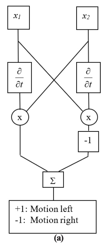
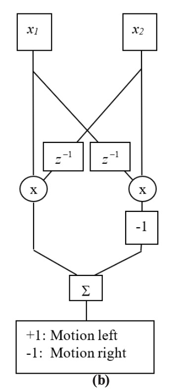
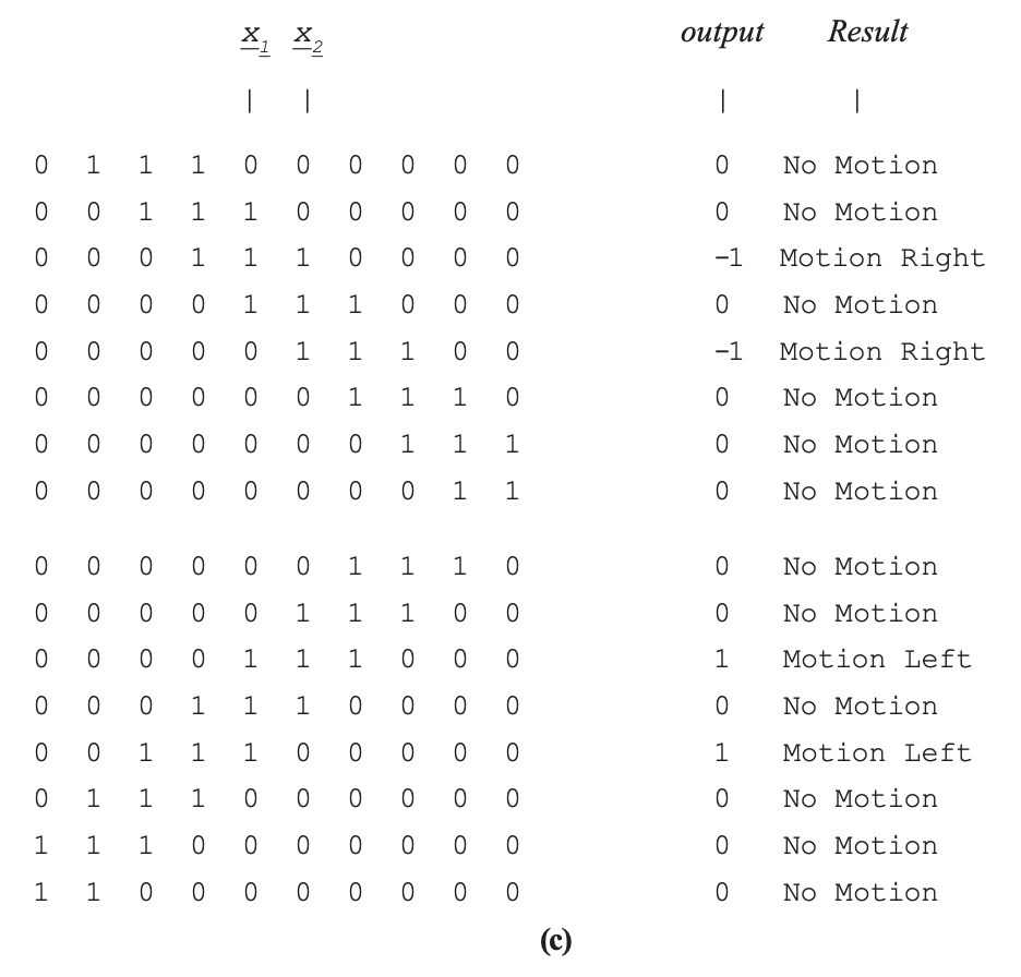
Figure 2.3.9–1. Hassenstein-Reichardt Motion Detectors.
Two implementations shown: (a) in-channel differentiators, and (b) cross-channel delays. (c) MATLAB simulation results are the same for both implementations.
Exercise 2.3.9-1
Give the expected output (Right, Left or No Motion) of a two-element Hassenstein-Reichardt motion detector given the following two input sequences; assume all previous values are zero. Either model (in-channel derivatives or cross-channel delays) should give the same results:
| Sequence 1 | Sequence 2 |
| x1 x2 Output | x1 x2 Output |
| 0 0 No Motion | 0 0 No Motion |
| 0 0 __________ | 1 0 __________ |
| 1 1 __________ | 0 1 __________ |
| 0 0 __________ | 0 0 __________ |
| 1 0 __________ | 0 1 __________ |
| 0 1 __________ | 1 1 __________ |
| 1 0 __________ | 1 0 __________ |
| 0 0 __________ | 0 0 __________ |
Answers:
| Sequence 1 | Sequence 2 |
| x1 x2 Output | x1 x2 Output |
| 0 0 No Motion | 0 0 No Motion |
| 0 0 No Motion | 1 0 No Motion |
| 1 1 No Motion | 0 1 Motion Right |
| 0 0 No Motion | 0 0 No Motion |
| 1 0 No Motion | 0 1 No Motion |
| 0 1 Motion Right | 1 1 Motion Left |
| 1 0 Motion Left | 1 0 Motion Left |
| 0 0 No Motion | 0 0 No Motion |