4.1: Water Budgets for Sustainable Water Management

Stacy L. Hutchinson

Kansas State University

Biological and Agricultural Engineering

Manhattan, Kansas, USA

Key Terms

Hydrologic cycle	Infiltration and runoff	Water balance
Soil water relationships	Evapotranspiration	Agricultural water management
Precipitation	Water storage	Urban stormwater management

Variables

• θ_g = gravimetric water content
• θ_v = volumetric water content
• ρ_b = bulk density of the soil
• AW = available water
• E = Evaporation
• ET = evapotranspiration
• DS = deep seepage
• FC = field capacity
• In = Infiltration
• Ir = irrigation
• PWP = permanent wilt point
• P = precipitation
• R = net runoff (R_in – R_out)
• R_in = runoff into the area of interest
• R_out = runoff out of the area of interest
• T = Transpiration
• ∆S = change in soil water storage

Introduction

Water is central to many discussions regionally, nationally, and globally—be it the lack of water, the overabundance of water, or poor water quality—pushing us to seek answers on how to ensure we can maintain a safe, reliable, adequate water supply for human and environmental well-being. The United Nations (2013) defines water security as

. . . the capacity of a population to safeguard sustainable access to adequate quantities of acceptable quality water for sustaining livelihoods, human well-being, and socio-economic development, for ensuring protection against water-borne pollution and water-related disasters, and for preserving ecosystems in a climate of peace and political stability . . .

This highlights the need to understand the complex relationships associated with water and the need to research, develop, and implement engineered systems that assist with enhancing water security across the nation and world. This chapter focuses on understanding the system water balance, which is the fundamental basis for all water management decisions.

Outcomes

After reading this chapter, you should be able to:

• • Describe the basic components of a water balance, including precipitation, infiltration, evaporation, evapotranspiration, and runoff
• • Calculate a water budget
• • Use a water budget for the design and implementation of a simple water management system for irrigation or sustainable stormwater management

Concepts

Hydrologic Cycle

Hydrology is the study of how water moves around the Earth in continuous motion, cycling through liquid, gaseous, and solid phases. This cycle is called the hydrologic cycle or water cycle (Figure 3.4.1). At the global scale, the hydrologic cycle can be thought of as a closed system that obeys the conservation law; a closed system has no external interactions. The vast majority of water in the system continues to cycle through the three states of matter: liquid, gaseous, and solid.

Key processes in the hydrologic cycle are:

• • Precipitation (P), which is the primary input into a water budget. Precipitation describes all forms of water (liquid and solid) that falls or condenses from the atmosphere and reaches the earth’s surface (Huffman et al., 2013), including rainfall, drizzle, snow, hail, and dew.
• • Infiltration (In), which is the movement of water into the soil. Infiltrated water from precipitation and irrigation are the primary sources of water for plant growth.

Figure \(\PageIndex{1}\): The water cycle, hydrologic cycle (USGS, 2020a).

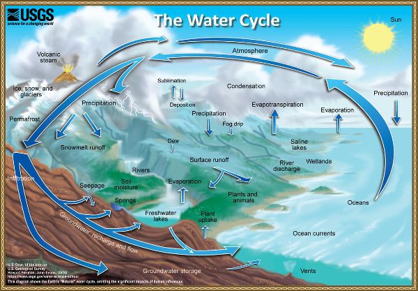
• • Evaporation (E), which is the conversion of liquid or solid water into water vapor (gaseous water).
• • Transpiration (T), which is the process through which plants use water. Water is absorbed from the soil, moved through the plant, and evaporated from the leaves.
• • Evapotranspiration (ET), which is the combination of evaporation and transpiration to describe the water use, or output, from vegetated surfaces.
• • Runoff (R), which is the precipitation water that does not infiltrate into the soil. Runoff is generally an output, or loss of water, from the system or area of interest, but can also be an input if this water runs into the system or area of interest.
• • Deep seepage (DS), which is water that infiltrates below the root zone, which is the depth of the area of interest for the water budget.

Soil Water Relationships

The design of water management systems by biosystems engineers involves water moving through or being held in the soil. Thus, soil-water dynamics are a critical factor in the design process.

A volume of soil is comprised of solids and voids, or pore space. Porosity is the volume of voids as compared to the total volume of the soil. The proportions of solids and voids depend on the soil particles (sand, slit, clay, organic matter) and structure (known as peds), with coarse-textured soils (i.e., dominated by sand) having approximately 30% voids and finer-textured soils (i.e., containing more silt or clay) having as much as 50% void space. Water that infiltrates into the soil profile is stored in the soil voids. When all the void space is filled with water, the soil is at saturation water content.

Figure \(\PageIndex{2}\): Graphical description of soil water.

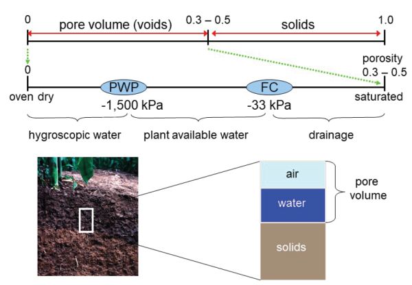
Gravitational forces remove water up to 33 kPa (1/3 bar) of tension; this is drainage or gravitational water. The soil water content after gravitational drainage for approximately 24 hrs is called field capacity (FC) and is the maximum water available for plant growth. At this point, water is held in the soil in the smaller pore spaces by capillary action and surface tension, and can be removed from the soil profile by plant roots extracting the water from those pores. The water tension of the soil at field capacity (the suction pressure required to extract water from the pore spaces) is around 10 kPa (0.1 bars) for sands to 30 kPa (0.3 bars) for heavier soils containing more silt or clay. Plants are able to extract water from the soil profile with up to 1,500 kPa (15 bars) of tension; the water content at 1,500 kPa (15 bars) of tension is called the permanent wilt point (PWP). The total plant available water (AW) for a given soil profile is the difference between FC and PWP:

\[ AW = FC - PWP \]

Plant water use is the primary means of removing water from the soil profile. Once all of the available water has been taken up by plants, some water remains in the soil, in very small pore spaces where very high suction pressure would be needed to remove that water. This film of water is more tightly bound to soil particles than can be extracted by plants and is called hygroscopic water. These relationships are shown in Figure 3.4.2.

The amount of water in the soil is called the soil water content or soil moisture content, and is often indicated using the symbol θ. When soil water content is expressed on a mass basis, i.e., mass of water in the soil compared to total mass of soil, it is called gravimetric water content (θ_g). Gravimetric water content can be calculated by expressing mass of water as a proportion of total wet mass of soil, known as wet weight water content, or as a proportion of total dry mass of soil, known as dry weight water content (Equation 3.4.2). When expressed on a volume basis, i.e., volume of water as a proportion of the total volume, with units cm_w³ cm⁻³, the value is called volumetric water content (θ_v) (Equation 3.4.3). Gravimetric (dry weight) and volumetric water content are related through the bulk density of the soil (ρ_b), which is the mass of soil particles in a given volume of soil, expressed in g cm⁻³.

\[ \text{gravimetric water content} (\Theta_{g}) = \frac{\text{mass water}}{\text{mass dry soil}} = \frac{\text{mass total soil - mass dry soil}}{\text{mass dry soil}} \]

\[ \text{volumetric water content} (\Theta_{v}) = \frac{\text{volume water}}{\text{total volume soil}} = \Theta_{g} \frac{\text{solid bulk density } (\rho_{b})}{\text{density of water }(\rho_{w})} \]

As collection of a known volume of soil is more difficult than collecting a simple grab sample of soil, it is much easier to determine gravimetric water content by mass. However, volumetric soil moisture is much easier to use in calculations because it can be expressed as an equivalent depth of rainfall (mm) over a given area and, thus, be directly related to rainfall, which is most commonly reported in units of depth (such as mm) and never in mass. The volume of water input to the water budget can be calculated by multiplying the depth of rainfall by the area receiving rain.

Water Budget Calculation

A water budget, or water balance, is a measure of all water flowing into and out of an area of interest, along with the change of water storage in the area. This could be an irrigated field, a lake or pond, or green infrastructure such as a stormwater management system like a bioretention cell or a rain garden (a vegetated area to absorb and store stormwater runoff). At smaller scales, the hydrologic cycle is characterized using a water budget, which is the primary tool used for designing and managing water resources systems, including stormwater runoff management and irrigation systems. Water budgets are calculated for a defined system or area (e.g., field, pond) over a specified time period (e.g., rainfall event, growing season, month, year).

Figure \(\PageIndex{3}\): Water balance.

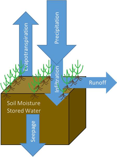
The water budget is calculated by quantifying the inputs, outputs, and change in water storage (∆S) of the system or project (Equation 4.1.4; Figure 4.1.3). While precipitation is the primary input to the water budget, others include runoff into the system (R_in) and water added through irrigation (Ir). Outputs from the system include runoff (R_out), deep seepage (DS), and evapotranspiration (ET). The change in system storage (∆S) may be positive, such as an increase in pond water level after a rainfall event, or negative, such as the decline in soil moisture from plant water use.

\[ P+Ir \ \pm R - ET - DS = \Delta S \]

where P = precipitation

Ir = irrigation

R = net runoff (R_in – R_out)

ET = evapotranspiration

DS = deep seepage

∆S = change in soil water storage

The first step in developing a water budget for water resources management is to collect input, output, and storage data. There are many sources of data for this, including the National Oceanic and Atmospheric Administration (NOAA) National Centers for Environmental Information (NCEI) (NOAA, 2019), which includes data from around the world. Within the U.S., the U.S. Geological Survey (USGS) real-time water data (USGS, 2020b) and the U.S. Department of Agriculture (USDA) Natural Resources Conservation Service (NRCS) Web Soil Survey (USDA-NRCS, 2019a) are also available. Each of these sources has extensive sets of data available to assist with management of water resources. Local-level data from state climatologists, research farms, and project gages should also be considered when available. High quality precipitation data are particularly valuable, and necessary, when designing and implementing water management systems including irrigation systems and green infrastructure.

Precipitation

Precipitation is the primary input into a water budget. The most important form of precipitation for agricultural and biological engineering applications in most parts of the world is rainfall. Precipitation varies significantly across regions (Figure 4.1.4) and throughout the year, but is relatively consistent over long time periods at a given location. This means long-term precipitation records can be used to calculate a water budget and for planning water resource management systems.

Figure \(\PageIndex{4}\): Mean annual precipitation (mm year^–1) for the 1980-2010 period from AgMERRA (from Ruane et al., 2015).

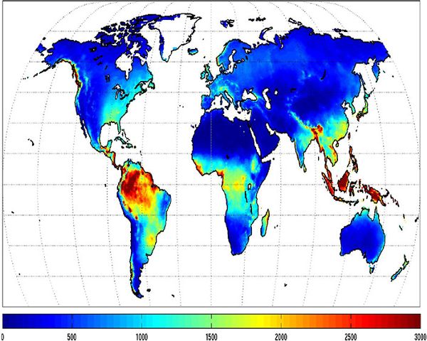
In addition to data available from NOAA NCEI and local sources mentioned above, long-term design storm information is available for the U.S. from the NOAA Atlas 14 point precipitation frequency estimates (HDSC, 2019). Statistical analysis of historic precipitation data is used to determine the magnitude and annual probability for various rainfall events. These values are used to size stormwater systems to deal with the majority of events, but not the most extreme.

Infiltration

Precipitation starts moving into the soil profile, i.e., infiltrating, as soon as it reaches the ground surface. Initial infiltration rates depend on the initial soil water content, but if the soil is drier than field capacity, can be very high as water fills depressions on the soil surface and begins moving into the soil. As the surface depressions fill and the surface soil becomes saturated, infiltration slows to steady-state and excess precipitation begins to run off the surface. Depending on the type of precipitation, initial soil water content, duration, and intensity (depth per time), precipitation may infiltrate into the soil profile and become soil water, or it will not infiltrate and will become runoff. The infiltration rate is related to soil bulk density, porosity, pore size distribution, and pore connectivity.

Runoff

Water that does not infiltrate into the soil is an output from the water budget (a loss from the water management system) unless the system is designed to collect it. The amount of runoff depends on land cover type, soil type, initial soil water content, and rainfall intensity; these four factors all interact and are not independent of each other. Land cover plays a significant role in determining the amount of runoff. Natural vegetated land usually has the highest infiltration rates. Infiltration rates decrease as natural land is converted to production land, due to increased compaction and changes in soil structure, and to developed land, due to impervious surfaces such as buildings and roads. Soil type also influences whether water can infiltrate. Soils with greater connected pore space will tend to generate less runoff. Initial soil water content is important because, if the soil is at or near saturation water content, the infiltration rate is more likely to be less than the rainfall rate. If rainfall rate is very high, runoff can occur even if the soil is quite dry. One of the most common methods for estimating likely surface runoff is the curve number method (USDA-NRCS, 2004). More information on the curve number method can be found in Chapter 10, Part 630, of the USDA-NRCS National Engineering Handbook (USDA-NRCS, 2004).

Evapotranspiration

Evapotranspiration (ET) is the primary means for removing water from the top of the soil system when plants are present. If there are no plants this loss will be confined to evaporation only. The amount of ET depends on the type and growth stage of the vegetation, the current weather, and soil water content at the location. The most accurate ET calculations involve an energy balance associated with incoming solar radiation and the mass transfer of water from moist vegetation surfaces to a drier atmosphere (Allen et al., 2005). ET is driven by solar radiation, but as the soil becomes drier, ET decreases. The relationship depends on the pore size distribution of the soil, so is regulated by the interaction of soil texture (sand, silt, and clay content) and structure (presence and type of soil peds).

Storage

Soils can store a significant amount of water and play an important role in controlling the rainfall-runoff processes, stream flow, and ET (Dobriyal et al., 2012; Meng et al., 2017). Available soil water influences productivity of natural and agricultural systems (Dobriyal et al., 2012). Understanding the available water stored in surface soils allows effective design and implementation of irrigation and stormwater management systems. The maximum storage is determined by the total porosity of the soil, which will be almost the same as the saturated water content. The ability of the soil to store more water at any given time is determined by the difference in current water content and saturated water content. These factors are influenced by soil texture, structure, porosity, and bulk density. More information about soils can be found from sources such as the FAO Soils Portal of the Food and Agriculture Organization of the United Nations (FAO, 2020), the European Soil Data Centre (https://esdac.jrc.ec.europa.eu/), and on the Web Soil Survey maintained by the USDA-NRCS (2019b).

Applications

Water is essential for life and critical for both food and energy production. With a finite supply of available fresh water and increasing global population demanding access to clean water for drinking, energy, and food production, proper water management is of the utmost importance. It is imperative to research, develop, and implement engineered systems that enhance local, regional, national, and global water security. Water balances are used in the design of systems to manage excess stormwater and to manage scarce available water in low-rainfall areas. Excess water management systems include components to retain and regulate runoff safely, while limited water management systems include components to provide irrigation water during dry seasons.

Urban Stormwater Management

As urbanization and land development occurs, the addition of impervious structures (roads, sidewalks, buildings) dramatically changes the hydrology of an area. Runoff volume linearly increases with increases in the impervious surface area. Hydrologic models and long-term stream flow monitoring show that, compared to pre-development, developed suburban areas have 2 to 4 times more annual runoff, and high-density areas have 15 times more runoff (Sahu et al., 2012; Suresh Babu and Mishra, 2012; Christianson et al., 2015). As runoff travels over pavement, rooftops, and fertilized lawns that make up much of the urban landscape, it picks up contaminants such as pathogens, heavy metals, sediments, and excess nutrients (Davis et al., 2001), creating both water quantity and water quality concerns.

Increases in the total volume of runoff from urban areas are caused not only by impervious structures. Even in low-density suburban areas where individual lots have large lawns and large public parks are created, current methods of construction and development greatly reduce the infiltration capacity of soils. Development typically involves stripping native vegetation from large areas of land, accelerating soil erosion rates 40,000 times (Gaffield et al., 2003). During this process, construction equipment compacts soil, reducing its ability to absorb runoff. Developed lawns can generate 90% as much runoff as pavement (Gaffield et al., 2003). Urban runoff may also include dry-weather flows from the irrigation of lawns and public parks. The final result of urban development is a significant increase in runoff that transports pollutants from dense urban centers to receiving water bodies, and small changes in land use can relate to large increases in flood potential and pollutant loading.

Over the past three decades, urban and urbanizing areas have started to increase the use of green infrastructure, or natural-based systems, for stormwater management. Green infrastructure works to reduce stormwater runoff and increase stormwater treatment on-site for floodwater and nonpoint, or diffuse, source pollution control using infiltration and biologically based treatment in the root zone. Green infrastructure is very different from traditional grey stormwater management systems, such as storm sewers. The more traditional grey systems use a centralized approach to water management, designed to quickly move runoff off the land and into nearby surface water with little to no storage or treatment. Green infrastructure is more resilient and can offer additional benefits, such as habitat, in developed and developing areas. For more information about green infrastructure see the U.S. Environmental Protection Agency (USEPA) green infrastructure webpage (USEPA, 2020).

Bioretention cells are one of the most effective green infrastructure systems. Bioretention cells are designed to infiltrate, store, and treat runoff water from impervious surfaces such as parking lots and roadways. Bioretention cells can be lined to prevent contaminants from moving into groundwater or unlined when there is no concern of groundwater contamination. Ideally, bioretention cells are designed to infiltrate and store the “first flush” rainfall event. (The first flush rainfall is the first 13-25 mm of rain that removes the majority of accumulated pollution from surfaces.) However, in many cases, there is not enough space to install such a large bioretention cell and the system is designed to fit the space in order to treat as much stormwater as possible.

Initial design and assessment of bioretention cell function is completed using a system water balance. Runoff from the impervious parking is directed toward stormwater management practices, like bioretention cells, where water infiltrates and is stored until removed from the soil (or growing media) through evapotranspiration.

Agricultural Water Management

Changing climate conditions, population growth, and urbanization present challenges for food supply. Agricultural intensification impacts local resources, particularly usable freshwater. This vulnerability is amplified by a changing climate, in which drought and variability in precipitation are becoming increasingly common. As a result, 52% of the world’s population is projected to live in regions under water stress by 2050 (Schlosser et al., 2014). Concurrently, varying water availability, along with limiting nutrients, will constrain future food and energy production.

Agricultural water management is key to optimizing crop production. The amount of water needed for crop growth depends on the crop type, location, and time of year, but averages roughly 6.5 mm day⁻¹ during the growing season (Brouwer and Heibloem, 1986). Depending on location, installation of runoff management systems such as terraces (ASAE S268.6 MAR2017) and grassed waterways (ASABE EP 464.1 FEB2016) (ASABE Standards, 2016, 2017) may be needed to manage excess rainfall and reduce flooding and erosion within fields. Design standards with specific design criteria are available from the ASABE Standards (https://asabe.org/Publications-Standards/Standards-Development/National-Standards/Published-Standards).

In addition to managing runoff from rainfall events, supplementing natural rainfall with irrigation water for crop production may also be required (sometimes in the same places). Maintaining available water for crop growth and development has a significant impact on crop yields. Irrigation system design and management rely on the use of detailed soil water balances to minimize water losses and optimize crop production. A daily water budget to account for all inputs and outputs from the system can be calculated.

Examples

Example \(\PageIndex{1}\)

Example 1: Calculating soil water content

Problem:

The following information is provided to determine the amount of available water storage in a soil profile. A soil sample collected in the field has a wet weight of 238 g. After drying at 105°C for 24 hrs, the soil sample dry weight is 209 g. Careful measurement of the soil sample determines the volume of the soil core is 135 cm³. Determine the available water storage, in both mass and volume basis, in the soil profile. (a) What was the original water content of the soil on a gravimetric basis (mass of water per total mass) and (b) on a volumetric basis (volume of water per volume of bulk soil)?

Solution

1. (a) Calculate the gravimetric water content using Equation 3.4.2:

\( \text{gravimetric water content } (\Theta_{g}) = \frac{\text{mass water}}{\text{mass dry soil}} = \frac{\text{total mass soil - dry soil mass}}{\text{dry soil mass}} \)

\( \text {mass water (g)} = 238 \text{ g total} - 209 \text{ g dry} = 29 \text{ g water} \)

\( \text {gravimetry water content} (\Theta_{g}) = \frac{29 \text{ g water}}{209 \text{ g dry}} = 0.139 \frac{\text{g water}}{\text{g dry}} = 13.9 \% \text{ water by mass} \)

1. (b) Calculate the volumetric water content using Equation 4.1.3:

\( \text{volumetric water content } (\Theta_{v}) = \frac{\text{volume water}}{\text{total volume}} \)

\( \text{volume of water} = \frac{\text{mass water}}{\text{density of water}} = \frac{29 \text{ g water}}{1 \text{ g per cm}^{3}} = 29 \text{ cm}^{3} \text{ water} \)

\( \text{volumetric water content } (\Theta_{v}) = \frac{29 \text{ cm}^{3} \text{ water}}{135 \text{ cm}^{3} \text{ dry}} = 0.215 \frac{ \text{cm}^{3} \text{ water}}{\text{cm}^{3} \text{ dry}} = 21.5 \% \text{ water by volume} \)

Example \(\PageIndex{2}\)

Example 2: Determining plant available water

Problem:

Plant available water is one factor that helps to determine the need for irrigation as well as the available water storage in bioretention cells. A field has an established grass cover. The grass has an effective root zone depth of 0.90 m. The soil is a fine sandy loam with FC = 23% (vol) and PWP = 10% (vol), as shown in the water balance diagram.

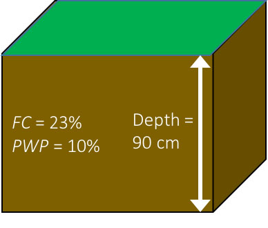
(a) If the soil is at field capacity, how much available water (cm) is in the effective root zone? (b) If the field water content averages 18% (vol) in the root zone, what is the available water storage depth for rainfall?

Solution

1. (a) Calculate the available water using Equation 4.1.1:

\( AW = FC - PWP = 23 \% \text{(vol)} - 10 \% \text{(vol)} = 13 \% \text{(vol)} \)

1. Thus, 13% of the soil volume is available water for plant use. When the volumetric water content is considered on a per unit area of soil, e.g., (cm³ water cm⁻² soil)/(cm³ soil cm⁻² soil), the units become depth water/depth soil, e.g. cm water cm⁻¹ soil profile. Thus, consider a unit area of soil and calculate the depth of available water:

\( \text{available water} = \frac{13 \text{ cm water}}{100 \text{ cm soil profile}} \times 90 \text{ cm} = 11.7 \text{ cm water available in root zone} \)

1. (b) If the soil water content is 18% (vol), calculate the available storage as the difference between FC and volumetric water content:

\( \text{available storage} = FC - \Theta_{v} = 23 \% - 18 \% = 5 \% \)

1. And the depth of available storage in the root zone is:

\( \text{depth of available storage} = 0.05 \times 90 \text{ cm} = 4.5 \text{ cm} \)

Thus, the soil profile would be able to store 4.5 cm in the 90 cm root zone.

Example \(\PageIndex{3}\)

Example 3: Using a water balance to design a simple pond to store runoff

Problem:

A developer is planning the layout of a small housing development on 16.2 ha (40 ac) of land near Manhattan, KS, USA. According to local ordinance, the developer must retain any increased runoff due to development from the 2-yr, 24-hr rainfall event (86 mm) (HDSC, 2019). Prior to development, the area was able to infiltrate and store approximately 50 mm of this rainfall event. With the increase of impervious land cover (e.g. houses and roads), it is expected that infiltration and storage will be reduced to 30 mm. Determine the pond volume required to store the difference in expected runoff.

Solution

Apply Equation 4.1.4 to the 16.2-ha site to determine the expected increase in runoff from the site to due development:

Water balance equation:

\( \text{inputs} - \text{outputs} = \text{change in storage} \)

\( P+Ir \pm R - ET-DS=\Delta S \)

Assumptions:

Pond is dry prior to rain

Ir = 0

ET = 0 for short duration events

DS = 0

Therefore, P ± R = ∆S

Pre-development:

P = 86 mm

R = ?

∆S = 50 mm

R = 86 mm – 50 mm = 36 mm of runoff

Post-development:

P = 86 mm

R = ?

∆S = 30 mm

R = 86 mm – 30 mm = 56 mm of runoff

Change in runoff:

∆S = 56 mm – 36 mm = 20 mm runoff

= 20 mm × 16.2 ha

= 0.02 m × 162,000 m² = 3,240 m³

The pond must be designed to detain, or slow down, 20 mm of runoff from the developed land. This equates to 3,240 m³ of runoff water from the entire development of 16.2 ha.

Example \(\PageIndex{4}\)

Example 4: Estimate the amount of storage available in a bioretention cell

Problem:

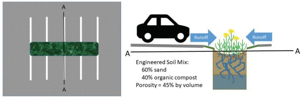
Consider a bioretention cell located in the center of a parking lot. The parking lot, an area of 26 m by 12 m, is sloped to direct runoff into the bioretention cell. The cell contains an engineered growing media that is 60% sand and 40% organic compost, with a porosity of 45% by volume, planted with native grasses and forbs. The cell is 2.0 m wide, 1.2 m deep, and 12 m long.

1. (a) What is the maximum water storage volume of the bioretention cell?
2. (b) What is the largest storm (maximum precipitation depth) the cell can infiltrate if all storage is available?

Solution

Solution:

1. (a) Calculate the total volume of the bioretention cell:
2. \( \text{volume of cell} = \text{length} \times \text{width} \times \text{depth} \)

= 12 m × 2 m × 1.2 m = 28.8 m³

1. The maximum storage is equal to the total void space (porosity):
2. \( \text{void space} = \text{volume of cell} \times \text{porosity} \)

= 28.8 m³ × 0.45 = 12.96 m³

1. (b) Assuming all rainfall will run off the parking lot, the maximum storm depth that can be stored is:
2. \( \text{rainfall} = \frac{\text{volume of cell void space}}{\text{area of parking lot}} = \frac{12.96m^{3}}{12m \times 26m} = 0.042m = 42mm \)
3. −1, preparing the cell to store the next rainfall event.

Example \(\PageIndex{5}\)

Example 5: Development of an irrigation schedule for corn in a water limited area

Problem:

Given the following information, determine the daily changes in the soil water content. How much irrigation water should be added on the 10^th day to raise the water content of the root zone back to the initial water content? The root zone is 1 m and the initial soil moisture content is 20% by volume. Assume all seepage passes through the root zone and is not stored.

Solution

Convert the initial soil amount in the profile at the beginning of day 1, θ_v = 20% of root zone, to units of depth of water in the root zone:

\( \theta_{vi} = 0.2 \times 1000 \ mm = 200 \ mm\text{ of water} \)

Apply Equation 4.1.4 to the root zone for each day:

\( \text{Daily water balance} = P+Ir \pm R-ET -DS=\Delta S \)

\( \text{Day 1 inputs} = P+Ir \pm R = 0+0+0=0\ mm \)

\( \text{Day 1 outputs} = R+ET+\text{seepage} = 0+7+0 = 7 \ mm \)

\( \text{Day 1 } \Delta S = \text{inputs} - \text{outputs} = 0\ mm - 7 \ mm = -7 \ mm \)

\( \text{Day 1 } \theta_{v1} = \theta_{vi} - \Delta S = 200 \ mm - 7 \ mm = 193 \ mm \)

There is 193 mm of water in the soil profile at the end of day 1.

It is easiest to complete the rest of these calculations by setting up a spreadsheet. The following table shows the daily water budget components, the summed inputs and outputs as calculated above, and the resulting soil water depth (mm) in the right-most column. Initial water = 200 mm. At water content is 183 mm. Thus, to return the amount of water in the profile to in the initial soil water content of 200 mm, 17 mm would need to be added on day 10.

Image Credits

Figure 1. USGS. (CC By 1.0). (2020). The water cycle. Retrieved from https://www.usgs.gov/media/images/water-cycle-natural-water-cycle

Figure 2. Hutchinson, S. L. (CC By 4.0). (2020). Soil water.

Figure 3. Hutchinson, S. L. (CC By 4.0). (2020). Water Balance.

Figure 4. Ruane et. Al. (2018). Annual Precipitation. Retrieved from https://data.giss.nasa.gov/impacts/agmipcf/

Figure 5. Hutchinson, S. L. (CC By 4.0). (2020). Example 2.

Figure 6. Hutchinson, S. L. (CC By 4.0). (2020). Example 4.

Figure 7. Hutchinson, S. L. (CC By 4.0). (2020). Example 5.

References

Allen, R. G., Walter, I. A., Elliott, R. L., Howell, T. A., Itenfisu, D., Jensen, M. E., & Snyder, R. L. (2005). The ASCE standardized reference evapotranspiration equation. Reston, VA: American Society of Civil Engineers.

ASABE Standards. (2016) EP 464.1: Grassed waterway for runoff control. St. Joseph, MI: ASABE.

ASAE Standards. (2017). S268.6: Terrace systems. St. Joseph, MI: ASABE.

Brouwer, C., & Heibloem, M. (1986). Irrigation water management: Irrigation water needs. Food and Agriculture Organization of the United Nations. Retrieved from http://www.fao.org/3/s2022e/s2022e00.htm#Contents

Christianson, R., Hutchinson, S., & Brown, G. (2015). Curve number estimation accuracy on disturbed and undisturbed soils. J. Hydrol. Eng., 21(2). http://doi.org/10.1061/(ASCE)HE.1943-5584.0001274.

Davis, A. P., Shokouhian, M., Sharma, H., & Minami, C. (2001). Laboratory study of biological retention for urban stormwater management. Water Environ. Res., 73(1), 5-14. doi.org/10.2175/106143001x138624.

Dobriyal, P., Qureshi, A., Badola, R., & Hussain, S. A. (2012). A review of the methods available for estimating soil moisture and its implications for water resource management. J. Hydrol., 458-459, 110-117. https://doi.org/10.1016/j.jhydrol.2012.06.021.

FAO. (2020). FAO soils portal. Food and Agriculture Organization of the United Nations. Retrieved from http://www.fao.org/soils-portal/en/.

Gaffield, S. J., Goo, R. L., Richards, L. A., & Jackson, R. J. (2003). Public health effects of inadequately managed stormwater runoff. Am. J. Public Health, 93(9), 1527-1533. https://doi.org/10.2105/ajph.93.9.1527.

HDSC. (2019). NOAA atlas 14 point precipitation frequency estimates. Hydrometeorological Design Studies Center. Retrieved from hdsc.nws.noaa.gov/hdsc/pfds/pfds_map_cont.html.

Huffman, R. L., Fangmeier, D. D., Elliot, W. J., Workman, S. R., & Schwab, G. O. (2013). Soil and water conservation engineering (7th ed.). St. Joseph, MI: ASABE.

Meng, S., Xie, X., & Liang, S. (2017). Assimilation of soil moisture and streamflow observations to improve flood forecasting with considering runoff routing lags. J. Hydrol., 550, 568-579. http://doi.org/10.1016/j.jhydrol.2017.05.024.

NOAA. (2019). Climate data online. National Oceanic and Atmospheric Administration, National Centers for Environmental Information. Retrieved from https://www.ncdc.noaa.gov/cdo-web/.

Ruane, A. C., Goldberg, R., & Chryssanthacopoulos, J. (2015) AgMIP climate forcing datasets for agricultural modeling: Merged products for gap-filling and historical climate series estimation, Agr. Forest Meteorol., 200, 233-248, http://doi.org/10.1016/j.agrformet.2014.09.016.

Sahu, R. K., Mishra, S., & Eldho, T. (2012). Improved storm duration and antecedent moisture condition coupled SCS-CN concept-based model. J. Hydrol. Eng. 17(11). https://doi.org/10.1061/(ASCE)HE.1943-5584.0000443.

Schlosser, C. A., Strzepek, K., Gao, X., Fant, C., Blanc, E., Paltsev, S., . . . Gueneau, A. (2014). The future of global water stress: An integrated assessment. Earth’s Future, 2(8), 341-361. doi.org/10.1002/2014EF000238.

Suresh Babu, P., & Mishra, S. (2012). Improved SCS-CN–inspired model. J. Hydrol. Eng. 17(11). https://doi.org/10.1061/(ASCE)HE.1943-5584.0000435

United Nations. (2013). Water security and the global water agenda. A UN-Water Analytical Brief. Retrieved from https://www.unwater.org/publications/water-security-global-water-agenda/.

USDA-NRCS. (2004). Chapter 10: Estimation of direct runoff from storm rainfall. In National engineering handbook, part 630 hydrology. U.S. Department of Agriculture Natural Resources Conservation Service. Retrieved from https://www.nrcs.usda.gov/wps/portal/nrcs/detailfull/national/water/manage/hydrology/?cid=STELPRDB1043063.

USDA-NRCS. (2019a). Web soil survey. USDA Natural Resources Conservation Service. Retrieved from https://websoilsurvey.sc.egov.usda.gov/App/HomePage.htm.

USDA-NRCS. (2019b). Soils. U.S. Department of Agriculture Natural Resources Conservation Service. Retrieved from https://www.nrcs.usda.gov/wps/portal/nrcs/main/soils/survey/.

USEPA (2020). Green infrastructure. U.S. Environmental Protection Agency. Retrieved from https://www.epa.gov/green-infrastructure.

USGS (2020a) The water science school. U.S. Geological Survey. Retrieved from https://water.usgs.gov/edu/watercycle.html.

USGS (2020b). National Water Information System: Web interface. U.S. Geological Survey. Retrieved from https://waterdata.usgs.gov/nwis.