3: Critical Properties and Acentric Factor

Last updated

Mar 5, 2021
Save as PDF
- 2: Vapor Pressure
- 4: New Vapor Pressure Equation

Larry Coleman
Consultant on Demand

$\newcommand{\vecs}[1]{\overset { \scriptstyle \rightharpoonup} {\mathbf{#1}} }$

$\newcommand{\vecd}[1]{\overset{-\!-\!\rightharpoonup}{\vphantom{a}\smash {#1}}}$

$\newcommand{\id}{\mathrm{id}}$ $\newcommand{\Span}{\mathrm{span}}$

( \newcommand{\kernel}{\mathrm{null}\,}\) $\newcommand{\range}{\mathrm{range}\,}$

$\newcommand{\RealPart}{\mathrm{Re}}$ $\newcommand{\ImaginaryPart}{\mathrm{Im}}$

$\newcommand{\Argument}{\mathrm{Arg}}$ $\newcommand{\norm}[1]{\| #1 \|}$

$\newcommand{\inner}[2]{\langle #1, #2 \rangle}$

$\newcommand{\Span}{\mathrm{span}}$

$\newcommand{\id}{\mathrm{id}}$

$\newcommand{\Span}{\mathrm{span}}$

$\newcommand{\kernel}{\mathrm{null}\,}$

$\newcommand{\range}{\mathrm{range}\,}$

$\newcommand{\RealPart}{\mathrm{Re}}$

$\newcommand{\ImaginaryPart}{\mathrm{Im}}$

$\newcommand{\Argument}{\mathrm{Arg}}$

$\newcommand{\norm}[1]{\| #1 \|}$

$\newcommand{\inner}[2]{\langle #1, #2 \rangle}$

$\newcommand{\Span}{\mathrm{span}}$ $\newcommand{\AA}{\unicode[.8,0]{x212B}}$

$\newcommand{\vectorA}[1]{\vec{#1}} % arrow$

$\newcommand{\vectorAt}[1]{\vec{\text{#1}}} % arrow$

$\newcommand{\vectorB}[1]{\overset { \scriptstyle \rightharpoonup} {\mathbf{#1}} }$

$\newcommand{\vectorC}[1]{\textbf{#1}}$

$\newcommand{\vectorD}[1]{\overrightarrow{#1}}$

$\newcommand{\vectorDt}[1]{\overrightarrow{\text{#1}}}$

$\newcommand{\vectE}[1]{\overset{-\!-\!\rightharpoonup}{\vphantom{a}\smash{\mathbf {#1}}}}$

$\newcommand{\vecs}[1]{\overset { \scriptstyle \rightharpoonup} {\mathbf{#1}} }$

$\newcommand{\vecd}[1]{\overset{-\!-\!\rightharpoonup}{\vphantom{a}\smash {#1}}}$

$\newcommand{\avec}{\mathbf a}$

$\newcommand{\bvec}{\mathbf b}$

$\newcommand{\cvec}{\mathbf c}$

$\newcommand{\dvec}{\mathbf d}$

$\newcommand{\dtil}{\widetilde{\mathbf d}}$

$\newcommand{\evec}{\mathbf e}$

$\newcommand{\fvec}{\mathbf f}$

$\newcommand{\nvec}{\mathbf n}$

$\newcommand{\pvec}{\mathbf p}$

$\newcommand{\qvec}{\mathbf q}$

$\newcommand{\svec}{\mathbf s}$

$\newcommand{\tvec}{\mathbf t}$

$\newcommand{\uvec}{\mathbf u}$

$\newcommand{\vvec}{\mathbf v}$

$\newcommand{\wvec}{\mathbf w}$

$\newcommand{\xvec}{\mathbf x}$

$\newcommand{\yvec}{\mathbf y}$

$\newcommand{\zvec}{\mathbf z}$

$\newcommand{\rvec}{\mathbf r}$

$\newcommand{\mvec}{\mathbf m}$

$\newcommand{\zerovec}{\mathbf 0}$

$\newcommand{\onevec}{\mathbf 1}$

$\newcommand{\real}{\mathbb R}$

$\newcommand{\twovec}[2]{\left[\begin{array}{r}#1 \\ #2 \end{array}\right]}$

$\newcommand{\ctwovec}[2]{\left[\begin{array}{c}#1 \\ #2 \end{array}\right]}$

$\newcommand{\threevec}[3]{\left[\begin{array}{r}#1 \\ #2 \\ #3 \end{array}\right]}$

$\newcommand{\cthreevec}[3]{\left[\begin{array}{c}#1 \\ #2 \\ #3 \end{array}\right]}$

$\newcommand{\fourvec}[4]{\left[\begin{array}{r}#1 \\ #2 \\ #3 \\ #4 \end{array}\right]}$

$\newcommand{\cfourvec}[4]{\left[\begin{array}{c}#1 \\ #2 \\ #3 \\ #4 \end{array}\right]}$

$\newcommand{\fivevec}[5]{\left[\begin{array}{r}#1 \\ #2 \\ #3 \\ #4 \\ #5 \\ \end{array}\right]}$

$\newcommand{\cfivevec}[5]{\left[\begin{array}{c}#1 \\ #2 \\ #3 \\ #4 \\ #5 \\ \end{array}\right]}$

$\newcommand{\mattwo}[4]{\left[\begin{array}{rr}#1 \amp #2 \\ #3 \amp #4 \\ \end{array}\right]}$

$\newcommand{\laspan}[1]{\text{Span}\{#1\}}$

$\newcommand{\bcal}{\cal B}$

$\newcommand{\ccal}{\cal C}$

$\newcommand{\scal}{\cal S}$

$\newcommand{\wcal}{\cal W}$

$\newcommand{\ecal}{\cal E}$

$\newcommand{\coords}[2]{\left\{#1\right\}_{#2}}$

$\newcommand{\gray}[1]{\color{gray}{#1}}$

$\newcommand{\lgray}[1]{\color{lightgray}{#1}}$

$\newcommand{\rank}{\operatorname{rank}}$

$\newcommand{\row}{\text{Row}}$

$\newcommand{\col}{\text{Col}}$

$\renewcommand{\row}{\text{Row}}$

$\newcommand{\nul}{\text{Nul}}$

$\newcommand{\var}{\text{Var}}$

$\newcommand{\corr}{\text{corr}}$

$\newcommand{\len}[1]{\left|#1\right|}$

$\newcommand{\bbar}{\overline{\bvec}}$

$\newcommand{\bhat}{\widehat{\bvec}}$

$\newcommand{\bperp}{\bvec^\perp}$

$\newcommand{\xhat}{\widehat{\xvec}}$

$\newcommand{\vhat}{\widehat{\vvec}}$

$\newcommand{\uhat}{\widehat{\uvec}}$

$\newcommand{\what}{\widehat{\wvec}}$

$\newcommand{\Sighat}{\widehat{\Sigma}}$

$\newcommand{\lt}{<}$

$\newcommand{\gt}{>}$

$\newcommand{\amp}{&}$

$\definecolor{fillinmathshade}{gray}{0.9}$

Distillation Science (a blend of Chemistry and Chemical Engineering)

This is Part III, Critical Properties and Acentric Factor of a ten-part series of technical articles on Distillation Science, as is currently practiced on an industrial level. See also Part I, Overview for introductory comments, the scope of the article series, and nomenclature. The goal of this article is to explain how the critical properties and acentric factor are used, and how they may be estimated when reliable values are not available.

As discussed in Part II, the more basic vapor pressure equations have limitations that prevent them from being used in many modern industrial distillation systems, specifically at higher pressures. The concepts in this article will be used in Part IV, to introduce an improved vapor pressure equation, which removes the limitations of basic vapor pressure equations.

To implement the more sophisticated VP relationships and inter-compare the constants in Part IV, experimentally measured P vs T data needs to be put into reduced form. This is done only with the knowledge of the critical point, which is that singularity on the saturation line where the liquid and vapor phases become one. The critical temperature and pressure are identified as T_c and P_c. At the critical point, the specific molar volume is V_c.

$T_{r} = T/T_{c} \label{3-1}$

$P_{r} = P/P_{c} \nonumber$

$V_{r} = V/V_{c} \nonumber$

(note that reduced properties have the advantage of being dimensionless)

Using reduced variables T_r, P_r and V_r from Equation ( $\ref{3-1}$ ) also allows introduction to the concept of the "Law of Corresponding States" ( which is really not a scientific law per se, but more of a generally followed relationship). This "law" expresses the generalization that those properties dependent on intermolecular forces are related to the critical properties in the same way for all fluids. This concept underlies the development of several later articles of this series on Distillation Science, including Parts IV through VII.

The critical compressibility is Z_c, as defined as:

$Z_{c}= \frac {P_{c}V_{c}}{RT_{c}} \label{3-2}$ which is also dimensionless.

Two other properties are important to note:

$T_b$ is defined as the atmospheric pressure boiling point of a fluid, with $T_{br}$ as the reduced value of the atmospheric boiling point
$ω$ is the acentric factor, which is a measure of molecular complexity as defined as:

$\omega=-\log_{10}(VP)-1 \label{3-3}$ where the VP (in atmospheres) is evaluated at T_r= 0.7

The term “acentric factor” comes from Kenneth Pfizer's observation in 1955 that compact and near-spherical molecules have close to zero values when their ω is calculated. For example, neon, argon and krypton have ω values of -0.04, 0.00 and 0.00, respectively (helium has a more slightly negative ω, the value depending on isotope). Methane (CH₄) has a ω of 0.011; and the molecularly larger silane (SiH₄) has an ω of 0.099. An even larger and more complex molecule, like carbon tetrachloride (CCl₄) has an ω of 0.193; whereas silicon tetrachloride (SiCl₄) has an ω of 0.248. So valuation of the acentric factor from VP data and knowledge of the critical point is a good validation check against the known molecular size and shape.

For Equations of State (see Part V) that are more advanced than Van der Waals, the acentric factor is a required property, along with critical temperature and pressure. It is also used along with critical properties in the estimation of binary interaction parameters in Part VII.

As mentioned in Part II, the basic VP relationships have acceptable accuracy to obtain good values of T_bfrom available data. Experimental data is often taken near atmospheric pressure, but not exactly at one atmosphere absolute (i.e, 760 mmHg = 760 Torr = 101.325 Pa). Instead of blindly accepting a value of T_bfrom a handbook or single website, the practicing scientist or engineer should consider the data’s source and reliability. There is ready internet availability of atmospheric boiling points, critical property data, and acentric factors, especially on the NIST WebBook and global websites like Dechema, Infotherm (recently acquired by John Wiley and Sons from FIZ Chemie Berlin).

A recommended way to sort through the dizzying amount of critical property data (i.e., T_c , P_c, and V_c) is to use the correlation techniques of Lyderson ("Estimation of Critical Properties of Organic Compounds", University of Wisconsin College of Engineering, 1955) and others, which are specifically geared toward organic compounds. With some algebraic manipulation and adjustment of Lyderson’s parameters (since the usage intent here is for polar compounds that are not organic, but are not ionic either), and based on data across homologues, the following relationships seem to hold and are recommended for both validating questionable data or filling in “holes” of no data:

For T_b, the general correlating relationship within a homologue ( e.g., from silane to silicon tetrachloride, or from phosphine to trichlorophosphine) :

$(T_{b}\times MW)^n= A+B\times MW \label{3-4}$

where MW is the molecular weight. For chlorosilanes, chloromethanes, chlorophosphines, etc, this relationship shows a best fit with an exponent “n” of 0.8320. The constants A and B for the homologue are typically set by the hydride and chloride, since that data is usually more reliable. Where the core atom is not just carbon or silicon, but a blend (i.e, a methyl silane), an exponent of 0.8455 fits the data a bit better. This contrasts with organic compounds, whose data tends to fit best with somewhat lower exponents that are closer to 0.80.

For T_c(critical temperature), the best correlation within a homologue is found to be:

$\frac {T_{c}-T_{b}}{T_{c}}= A+B\times MW \label{3-5}$

where MW is the molecular weight and the constants A and B for the homologue are typically set by the hydride and chloride, as long as there is no organic content and the fluids are monomeric.

For P_c (critical temperature), use

$(\frac {MW}{P_{c}})^n= A+B\times MW \label{3-6}$

where MW is the molecular weight, exponent "n" = 0.5672, and constants A and B for the homologue are typically set by the hydride and chloride (as long as there is no organic content and the fluids are monomeric). For a pure organic compound, the exponent "n" should be Lyderson’s suggested 0.5000; for methyl silanes (e.g, dimethyl silane) the best exponent is 0.4550; and for Group III (dimeric bridge-bonded) compounds the best exponent fit is 1.03-1.08 ( 1.03 for di-gallanes and 1.08 for diboranes).

For V_c (critical molar volume), Lyderson’s rule of

$V_{c}=A+B\times MW \label{3-7}$

is probably still the best, where MW is the molecular weight and constants A and B for the homologue are typically set by the hydride and chloride. For some homologues, there is a possibility that the Vc vs MW relationship is not exactly linear, but rather has a slight concave quadratic nature; but the data is rarely good enough to determine such. Of all the critical properties, V_c is the hardest to experimentally measure, and is frequently estimated.

There is a way to get around some of the uncertainty with V_c, and that is to validate (or make minor V_cadjustments) based on the pattern of Z_cvalues in the homologue where

$Z_{c}= \frac{P_{c}\times V_{c}}{R\times T_{c}} \label{3-8}$

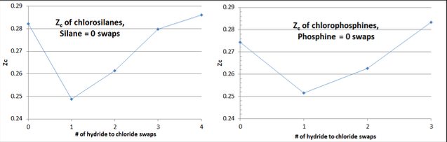
Within each homologue there is a characteristic “check-mark” pattern to Z_cvalues, when plotted against the number of hydrogen to chlorine swaps of the homologue (i.e., the homologue’s hydride has zero swaps, the monochloride one swap, the dichloride two swaps, etc). See below example data plot Figure 3-1 for the chlorosilane and chlorophosphine homologues.

The homologue’s hydride (which tends to be a fairly spherical shaped molecule with minimal dipole moment) typically has a Z_cin the range of 0.27-0.29. The first swap replaces a small “H” atom with a larger “Cl” atom, and re-orients the molecular shape to have a significant dipole, dropping the Z_cvalue by about 10%. Then the next swaps reduce the dipole, until the molecular shape returns closer to spherical, although significantly larger in diameter. Typically the Z_cof the completely chlorinated homologue fluid has a slightly larger Z_cthan the homologue’s hydride.

Screen Shot 2019-02-17 at 11.23.01 AM.png — Figure 3-1, Comparison of Z_c pattern within two homologues

To the extent that this “checkmark” shape is not observed in plotting calculated Z_c values per Equation 3-8, the “culprit” is almost always the value of V_c, which allows for some correction. The value of Z_cis known to have a significant relationship to molecular shape and complexity, although the stronger relationship between Z_cand the acentric factor, ω, is not so easily generalized as in organic compounds.

The importance of accurate values of T_b, T_c , P_c (and ω to an extent) is in calculating vapor pressure using the advanced relationship of Part IV. Having an accurate value of ω is more important, along with T_c, P_cin calculating the Equation of State for a fluid, in Part V. Having good values for ω and V_c are important to the estimation of binary interaction parameters in Part VII.

When two different types of swaps are made in a slightly polar molecule, an alternate technique is used to best correlate fluid properties (T_b , T_c , P_c , V_c, and ω), with a good example being methyl chlorosilanes. With methyl chlorosilanes, one or more methyl groups are substituted for hydrogen atoms (i.e., Si-H swapped to Si-CH₃), with the remaining Si-H bonding possibly swapped to Si-Cl. Another example would be swapping C-H for C-Cl and C-F bonding in chloro-fluoro methanes. There is no concise formula that governs such a dual substitution. Instead the concept of neural networks is used.

In this technique, the two base curves are laid out from the same starting compound (silane in the example below), and on each base curve the pertinent physical property values shown for each substituted homologue (chlorosilanes and methyl silanes being the base curves in the example below) vs molecular weight. For each amount of combined substitution (100%, 75% and 50% substitution = 0%, 25%, and 50% Si-H remaining) the data points are connected to their respective base curves. For example, on the 75% substitution amount, one would curve-connect trichlorosilane, methyl dichlorosilane, dimethyl monochlorosilane, and trimethyl silane.

Additional curve-connections could be made for values of constant amount of chlorine or methyl substitution (e.g., curve-connecting monochlorosilane, methyl monochlorosilane, dimethyl monochlorosilane, and trimethyl monochlorosilane). Using this method, the data on the dual-substituted fluids can be validated and adjustments made so that the curve-connections are smooth.

In the example in below Figure 3-2, the values of P_cfor methyl monochlorosilane (sic, me-mono) and dimethyl monochlorosilane (sic, di-me mono) are hardened up from rough measurements.

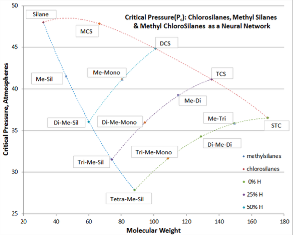
Screen Shot 2019-02-17 at 11.24.41 AM.png — Figure 3-2, Neural Network for methyl chlorosilanes’ P_cvalues

The value of the neural network technique is to make adjustments where data is poor or the estimation is of questionable accuracy. The presumption of neural networks is that for a class of compound, the continuum of structural changes should be uniform and internally consistent (although not necessarily linear).

Neural networks were constructed for all the pertinent properties of methyl chlorosilanes, and the technique found to be rather simple to deal with graphically using MS Excel. The resulting values were included in Table 3-3 below, for chlorosilanes and their common impurities, whose properties were validated using the correlating techniques of Equation ( $\ref{3-4}$ ) through Equation ( $\ref{3-8}$ ).

Table 3-3, Key properties, arranged by Group and Homologue
Fluid	MW	T_b	T_c	P_c	V_c	Z_c	ω
Group III(A)
B₂H₆	27.670	180.54	289.70	39.58	173.10	0.2882	0.1254
B₂H₅Cl	62.119^ǂ	216.37	346.33	37.13	189.92	0.2481	0.1283
BH₂Cl as monomer	42.284	237.72	379.56	37.10	206.73	0.2463	0.1315
BHCl₂ as monomer	82.722	266.07	422.71	37.63	240.37	0.2608	0.1389
B₂HCl₅hypothetic	199.893^ǂ	276.67	438.47	37.92	257.18	0.2711	0.1433
BCl₃	117.169	285.88	451.95	38.20	274.00	0.2822	0.1468
AlCl₃ as monomer	133.341	466.86^*	625.70	26.00	261.80	0.1326	0.3474
Ga₂H₄Cl₂ as dimer	214.383^ǂ	350.86	545.93	40.94	231.9	0.2120	0.2726
Ga₂H₂Cl₄ as dimer	283.273^ǂ	421.79	639.69	41.02	247.5	0.1943	0.3525
Ga₂Cl₆ as dimer	352.162^ǂ	473.49	694.00	37.70	263.0	0.1741	0.4504
Group IV(A)
SiH₄	32.117	161.75	269.65	47.99	130.07	0.2821	0.09860
SiH₃Cl	66.562	242.75	396.65	47.82	169.32	0.2488	0.1252
SiH₂Cl₂	101.007	281.45	449.45	44.83	215.05	0.2614	0.1589
SiHCl₃	135.452	306.15	479.15	41.15	267.28	0.2797	0.2090
SiCl₄	169.896	330.72	506.95	36.50	326.00	0.2860	0.2482
SiH₃(CH₃)	46.144	216.48	348.35	41.53	185.20	0.2691	0.1264
SiH₂Cl(CH₃)	80.589	278.82	439.11	41.16	233.90	0.2672	0.1793
SiHCl₂(CH₃)	115.034	314.17	489.18	39.25	287.81	0.2814	0.2269
SiCl₃(CH₃)	149.479	339.72	517.61	35.86	345.70	0.2919	0.2655
SiH₂(CH₃)₂	60.169	252.86	399.17	36.05	245.84	0.2706	0.1604
SiHCl(CH₃)₂	94.615	305.30	471.35	35.94	300.32	0.2791	0.2264
SiCl₂(CH₃)₂	129.061	342.89	519.21	34.26	358.20	0.2880	0.2740
GeH₄	76.642	184.93	307.98	54.77	128.28	0.2780	0.1270
GeH₃Cl	111.087	302.91	495.10	49.95	180.17	0.2215	0.1476
GeH₂Cl₂	145.532	334.60	536.93	45.36	236.71	0.2437	0.1721
GeHCl₃	179.976	343.54	541.41	41.42	283.96	0.2647	0.2012
GeCl₄	214.421	357.28	553.16	38.10	335.86	0.2819	0.2334
SnH₄	122.742	221.07	360.20	51.70	152.90	0.2674	0.1619
SnCl₄	260.521	387.21	591.85	36.95	351.20	0.2672	0.2625
Group V(A)
PH₃	33.998	185.41	324.75	64.51	113.33	0.2743	0.03052
PH₂Cl	68.443	273.09	463.73	62.29	153.63	0.2515	0.0750
PHCl₂	102.888	318.44	524.74	55.82	202.52	0.2625	0.1362
PCl₃	137.333	349.25	558.95	50.00	260.00	0.2834	0.2117
POCl₃	153.331	379.00	605.21	47.59	276.00	0.2645	0.1993

Table 3-3, Continued

AsH₃	77.945	210.73	373.00	65.12	132.50	0.2819	0.01341
AsH₂Cl	112.390	300.41	515.99	64.33	174.85	0.2657	0.0573
AsHCl₂	146.835	359.66	600.00	61.57	218.29	0.2730	0.1153
AsCl₃	181.281	403.30	654.00	58.35	259.56	0.2822	0.1875
SbH₃	124.781	256.09	446.20	66.61	157.20	0.2860	0.01659
SbCl₃	228.115	794.05	794.05	68.85	268.00	0.2832	0.3309
n-pentane	72.149	309.16	470.05	32.86	310.0	0.2641	0.2393
iso-pentane	72.149	300.82	460.56	33.17	307.1	.2695	0.2147

In above Table 3-3, those entries that are marked with a ^ǂ have their molecular weight given as the dimer. For AlCl₃, the asterisk on the T_bentry is for the best correlating value for the Part IV VP equation, even though it is below the triple point. Group IIIA compounds can feature “bridge-bonding” and can be either monomeric or dimeric. The two pentane entries at the end of the table are included because of their significance as electronic impurities, and to show that the techniques can be extended to organics.

With Group IIIA, some compounds are not included in a homologue simply because they are impossible structurally or are unstable. An example would be B₂H₃Cl₃, which would put too much strain on the B-B bridge-bond. Another is AlH₃ which cannot exist as a stand-alone liquid with vapor pressure at normal processing conditions, but tends to form stable hydrides with Group I metals such as LiAlH₄. However, B₂HCl₅is included (but noted as hypothetic), since some researchers claim to have seen its presence in low levels of TCS.

Search

Text Color

Text Size

Margin Size

Font Type

Distillation Science (a blend of Chemistry and Chemical Engineering)

Support Center

How can we help?