4: New Vapor Pressure Equation

Distillation Science (a blend of Chemistry and Chemical Engineering)

This is Part IV, New Vapor Pressure Equation of a ten-part series of technical articles on Distillation Science, as is currently practiced on an industrial level. See Part I, Overview for introductory comments, the scope of the article series, and nomenclature. Parts II and III are pre-requisite to Part IV.

Previous Part II, Vapor Pressure deals with the pure component equations normally found in textbooks, but which have limitations in industrial application. Part III, Critical Properties and Acentric Factor develops those parameters used to inter-relate conventional units of temperature, pressure and volume to their reduced property equivalents, as well as the Pfizer acentric factor that is used in modern Equations of State.

Several thermodynamically consistent vapor pressure (VP) equation forms have been developed in the past purposely for organic fluids, and typically have the stipulation that they do not work with either polar or heavily hydrogen-bonded fluids. Being both slightly polar in nature as well as hydrogen-bonded, chlorosilanes and their impurities fall exactly in this exclusion, and therefore make good continuing examples.

In this article, temperature and pressure are used in their reduced form, since this allows better inter-comparison between fluids, is dimensionless, and allows a more global future development. The reduced form is obtained by simply dividing conventional temperature, T, by the fluid’s critical temperature=> T_r = T/T_c. Similarly, reduced pressure is conventional pressure divided by the fluid’s critical pressure => P_r= P/P_c. Temperature and pressure must be in absolute units ( e.g., ºK not ºC)

Referring back to Part II, Equation 2-4, the Clausius-Clapeyron equation is given in reduced format, using \(\psi \nonumber\) as notation for the thermodynamic-based derivative of the natural log of (reduced) vapor pressure with respect to the inverse of (reduced) absolute temperature:

\[\psi = \frac{-d(\ln P_{r})}{d(1/T_{r})} = \frac{\Delta H_{v}}{\Delta ZRT_{c}} \label{4-1} \]

In order to have an improved VP equation form that can be used for the wide range between T_b and T_c (i.e., from atmospheric pressure to the critical point), that relationship should meet the following criteria:

1. The equation form should exactly have a reduced VP value of 1/P_c at T_b/T_c (i.e., yields the known atmospheric boiling point at atmospheric pressure), which is a well-measured lab value and is readily estimated based on structural considerations (see Part III article).
2. The equation form should exactly have a reduced VP value of unity at the critical temperature (i.e., match the measured value of the critical point), where the liquid meniscus disappears. This property can also be readily estimated based on structural considerations (see Part III article).
3. Give a reasonable value for reduced VP at T_r=0.7, corresponding to the definition of the Pfizer acentric factor, which has a basis in molecular complexity (see Part III article).
4. Meet the two thermodynamic consistency Reidel tests, as the critical point is approached ( that "α" monotonically drop to its lowest value at critical, and that the temperature derivative of α = zero at critical). See the left-most part of Equation (\ref{4-4}) for the definition of "α".
5. It must be noted that while this new vapor pressure relationship exactly matches the known atmospheric pressure boiling point, its differential form will not yield the known atmospheric pressure latent heat of vaporization

.Such a VP equation form would allow evaluation of modern Equations of State (see Part V article), Fugacity considerations (see Part VI article), and Binary Interaction Parameters (see Part VII article). Preferably the VP equation form would reasonably fit most fluids (both naturally occurring as well as synthetic), including polar compounds and those with substantial hydrogen bonding. Note that the VP equations given in Part II work over only narrow ranges; however above criteria #1 and #2 require the VP equation form to span a very broad range. In the text "The Properties of Gases and Liquids", by Prausnitz, et al, several alternate VP equation forms are discussed, all of which meet the above four criteria.

In his doctoral thesis at Syracuse University in 1965, under the guidance of Leonard Stiel, Richard Thek proposed exactly such an equation form to fill the technology gap. It was subsequently published by the AIChE in 1966. Unfortunately the computing power at that time was very limited, so equation forms with iterative solutions could not be used; and the internet did not exist to allow ready access to global data taken over the last many decades. Using modern computer processing speed and programming, these limitations have been resolved, and the constants determined for all chlorosilanes and their electronic impurities.

As given by Equation (\ref{4-2}) below, the original Thek-Stiel VP equation in its differential form has two terms: the first that governs at lower pressures close to atmospheric, and the second that takes over as the critical point is approached. While Thek set variables “q” and “k” equal to constants in order to avoid iterative solutions, with modern programming these can now be evaluated as true variables. The derivation of the final Modified Thek-Stiel VP Equation is available on request, but is not reproduced in these articles for the sake of brevity.

\[\frac{d(\ln P_{r})}{d(1/T_{r})} = \frac{A}{T_{r}^2}[1-B_{1}T_{r}+B_{2}T_{r}^2-B_{3}T_{r}^3+B_{4}T_{r}^4...]+ \frac{c}{T_{r}^2}(T_{r}^n-k) \label{4-2} \]

The several “B” constants result from the binomial expansion of the general Watson relationship for ΔH_v. After dropping the B₄ and higher expansion terms as non-significant mathematically and integrating, the resulting reduced vapor pressure equation is:

\[ \ln (P_{r})= A[B_{0}-T_{r}^{-1}-B_{1}\ln T_{r}+B_{2}T_{r}-(1/2)B_{3}T_{r}^2]+c\left[\frac{T_{r}^{n-1}-1}{n-1} +k(T_{r}^{-1}-1)\right] \label{4-3} \]

• \(A=\dfrac{\Delta H_{vb}}{RT_{c}(1-T_{br})^q} \nonumber\)
• \(B_{0}=1-B_{2}+(\frac{1}{2})B_{3} \nonumber\)
• \(B_{1}=q \nonumber\)
• \(B_{2}= \dfrac{q(q-1)}{2!} = \dfrac{q(q-1)}{2} \nonumber\)
• \(B_{3}=\dfrac{q(q-1)(q-2)}{3!} = \dfrac{q(q-1)(q-2)}{6} \nonumber\)
• \(c=\dfrac{\alpha_{c} -A(1-B_{1}+B_{2}-B_{3})}{1-k} \nonumber\)
• \(n=(1-k)+\dfrac{A}{c}(1-B_{2}+2B_{3}) \nonumber\)

The valuation of equation parameters ΔH_vb, q, k, and α_c are done iteratively using the techniques in Part X, Convergence Strategy, based on vapor pressure data, the molecule’s structure, and the value of T_br (the reduced atmospheric boiling point, T_b/T_c= T_br). P_r must be unity at the critical point (T_r= 1), which allows valuing the integration constant of Equation 4-3. The two important thermodynamic derivative functions are:

\[\frac{d(\ln P_{r})}{d(\ln T_{r})} = \alpha = A(T_{r}^{-1}-B_{1}+B_{2}T_{r}-B_{3}T_{r}^2)+c(T_{r}^{n-1}-\frac{k}{T_{r}}) \label{4-4} \]

\[\frac{-d(\ln P_{r})}{d(1/T_{r})} = \frac{\Delta H_{v}}{\Delta ZRT_{c}}= \psi = A(1-B_{1}T_{r}+B_{2}T_{r}^2-B_{3}T_{r}^3)+c(T_{r}^n-k) \label{4-5} \]

The "A" and "B" constants of Equations (\ref{4-2}), (\ref{4-3}), and (\ref{4-4}) are the same as Equation (\ref{4-5}). The evaluation of the Reidel derivative function "α" in Equation (\ref{4-4}) is used to establish thermodynamic consistency, and allows valuing an equation parameter. Note that the Clapeyron derivative of Equation (\ref{4-5}), \(\psi \nonumber\), is mathematically identical to that in Equation (\ref{4-1}). \(\psi \nonumber\) will be used Part V to establish the latent heat, ΔH_v, as well as the saturated vapor and liquid density of the fluids at the various conditions in the distillation column modeling.

Using the results of Part III, the Modified Thek-Stiel VP Equation constants are given below in Table 4-1, for chlorosilanes and electronic impurities found in the manufacture of high purity silicon. For brevity, the values of acentric factor, ω, and the critical Riedel derivative, \(\alpha_{c} \nonumber \), are not given in the table. They can be calculated from the other equation constants. In some instances, an electronic impurity can have either monomeric or dimeric form, but the form is noted in the table. Where a compound is not stable, the reader will note a “hole” in the table (e.g., AlH₃ and Ga₂H₆ are not stable as liquids or vapors).

Because the solution to the Modified Thek-Stiel VP Equation is necessarily iterative, the application of this VP relationship requires the use of some modern computing tools to perform such iterative calculations (aka “nested loops”). Depending on preference, this could be done as a macro in a spreadsheet program like MS Excel, or a stand-alone program developed in BASIC (or MatLab or Fortran). As mentioned above, some tips on convergence strategy are given in Part X.

Table 4-1 is rather expansive, to illustrate how general the new VP relationship is. Table organization is primarily done by Periodic Table Group (e.g., Group III, Group IV, and Group V) of the molecule’s core atom, and then by the homologue from hydride to chloride. Methyl chlorosilanes are included as examples of good application to fluids that form the border between classically organic and inorganic. Two of the pentanes are included, which happen to be of industrial concern as electronic impurities, to illustrate that the new VP equation is useful for organic fluids as well.

While volatile Group II, Group VI and Group VII fluids seem to follow the new VP relationship as well, there are no entries given in Table 4-1 since these fluids are generally not of concern in the production of electronic materials. The reader is encouraged to follow the evaluation techniques and stratagems given in these articles to further develop use of the new VP equations.

Table 4-1, VP solution constants, by Group and Homologue

Fluid	MW	A	B0	B1	B2	B3	c	n	k
Group III(A)
B2H6	27.670	8.9910	1.1494	0.37848	-0.11762	0.063573	2.8701	4.7796	0.1197
B2H5Cl	62.119^ǂ	8.1915	1.1494	0.37867	-0.11764	0.063578	3.4560	3.8431	0.1073
BH2Cl as monomer	42.284	8.3872	1.1495	0.37888	-0.11766	0.063583	3.2767	4.0925	0.0938
BHCl2 as monomer	82.722	8.9910	1.1495	0.37937	-0.11772	0.063596	2.7577	4.9953	0.0636
BCl3	117.169	9.5652	1.1496	0.37988	-0.11779	0.063609	2.2357	6.2975	0.0291
AlCl3 as monomer	133.341	11.9183	1.1512	0.39300	-0.11928	0.063892	2.2700	7.5185	0.0291
Ga2H4Cl2 as dimer	214.383^ǂ	7.0714	1.1506	0.38810	-0.11874	0.063799	5.3346	2.5583	0.0938
Ga2H2Cl4 as dimer	283.273^ǂ	10.8499	1.1513	0.39333	-0.11931	0.063898	3.3656	4.9567	0.0636
Ga2Cl6 as dimer	352.162^ǂ	11.1760	1.1520	0.39974	0.11997	0.063996	3.8566	4.5874	0.0291
Group IV(A)
SiH4	32.117	7.4652	1.1492	0.37673	-0.11740	0.063525	3.6247	3.4716	0.0914
SiH3Cl	66.562	8.8830	1.1494	0.37847	-0.11761	0.063572	2.7614	4.9286	0.0756
SiH2Cl2	101.007	9.9221	1.1497	0.38068	-0.11788	0.063629	2.1589	6.6627	0.0598
SiHCl3	135.452	9.9796	1.1501	0.38395	-0.11827	0.063708	2.5687	5.7950	0.0446
SiCl4	169.896	10.0240	1.1504	0.38651	-0.11856	0.063765	2.8465	5.3590	0.0291
SiH3(CH3)	46.144	9.0535	1.1494	0.37855	-0.11762	0.063574	2.6380	5.1963	0.0758
SiH2Cl(CH3)	80.589	10.1402	1.1499	0.38201	-0.11804	0.063662	2.1796	6.7338	0.0600
SiHCl2(CH3)	115.034	9.1805	1.1503	0.38512	-0.11840	0.063735	3.3346	4.3854	0.0446
SiCl3(CH3)	149.479	10.1187	1.1506	0.38512	-0.11840	0.063789	2.9357	5.2665	0.0291
SiH2(CH3)2	60.169	8.2747	1.1497	0.38077	-0.11789	0.063631	3.4554	3.9214	0.0603
SiHCl(CH3)2	94.615	9.1914	1.1503	0.38509	-0.11840	0.063734	3.3232	4.4012	0.0447
SiCl2(CH3)2	129.061	10.1007	1.1507	0.38820	-0.11875	0.063801	3.0279	5.1285	0.0291
GeH4	76.642	8.1986	1.1494	0.37858	-0.11763	0.063575	3.3615	3.9445	0.0914
GeH3Cl	111.087	8.6130	1.1496	0.37993	-0.11779	0.063610	3.1743	4.3025	0.0756
GeH2Cl2	145.532	8.8966	1.1498	0.38154	-0.11798	0.063650	3.1184	4.4929	0.0598
GeHCl3	179.976	9.1230	1.1501	0.38344	-0.11821	0.063696	3.1490	4.5641	0.0446
GeCl4	214.421	9.4041	1.1503	0.38554	-0.11845	0.063744	3.1654	4.6724	0.0291
SnH4	122.742	9.0298	1.1497	0.38087	-0.11790	0.063634	3.0671	4.5745	0.0914
SnCl4	260.521	10.1994	1.1506	0.38745	-0.11867	0.063744	2.8471	5.4354	0.0291
Group V(A)
PH3	33.998	7.8041	1.1485	0.37228	-0.11684	0.063396	2.8050	4.3644	0.1009
PH2Cl	68.443	8.6412	1.1490	0.37518	-0.11721	0.063482	2.4920	5.2267	0.0766
PHCl2	102.888	8.5412	1.1495	0.37919	-0.11770	0.063591	3.0719	4.3813	0.0527
PCl3	137.333	7.2366	1.1501	0.38413	-0.11829	0.063712	4.4289	2.9789	0.0291
POCl3	153.331	9.7746	1.1500	0.38331	-0.11819	0.063693	2.4586	5.9576	0

Table 4-2, VP solutions, by Group and Homologue, continued

Fluid	MW	A	B0	B1	B2	B3	c	n	k
Group V(A),cont’d
AsH3	77.945	7.4208	1.1484	0.37116	-0.11670	0.063362	2.9474	4.0298	0.1009
AsH2Cl	112.390	8.5242	1.1488	0.37403	-0.11707	0.063448	2.3972	5.3468	0.0766
AsHCl2	146.835	9.3548	1.1493	0.37782	-0.11754	0.063555	2.1821	6.2831	0.0527
AsCl3	181.281	10.0281	1.1499	0.38254	-0.11810	0.063675	2.2519	6.5171	0.0291
SbH3	124.781	8.5409	1.1484	0.37136	-0.11673	0.063368	2.0491	6.0821	0.1009
SbCl3	228.115	7.1200	1.1511	0.39192	-0.11916	0.063873	5.3455	2.6317	0.0291
n-pentane	72.149	10.0508	1.1504	0.38593	-0.11849	0.063753	2.6269	5.7673	0
iso-pentane	72.149	9.9797	1.1502	0.38432	-0.11831	0.063717	2.4514	6.0715	0

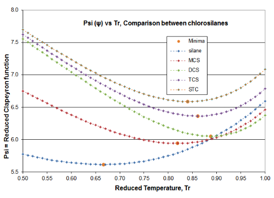
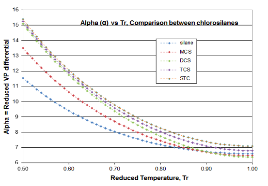
Two plots are offered in Figure 4-3 to validate the principles of this Distillation Science article. These plots are for the \(\psi \)(Psi) function of Equation (\ref{4-5}) and the \(\alpha \)(alpha) function of Equation (\ref{4-4}), for the chlorosilane homologue. The derivative function \(\phi \) goes through the required minimum, which produces the expected inflection in the vapor pressure curve, typically around T_r= 0.80-0.86. Silane’s minimum \(\phi \)occurs at T_r=0.67 and DCS’s minimum \(\phi \) occurs at T_r= 0.89. The fact that two fluids of this homologue are outliers illustrates why chlorosilane vapor pressures are so poorly fit by VP expressions that are intended for use with hydrocarbons. However, it can be seen how the Reidel \(\alpha \) function does fit the thermodynamic consistency requirements: for all homologue fluids, the \(\alpha \) function asymptotes to a constant value (\(\alpha_{c} \)) as the critical point is approached, with the slope of the \(\alpha \) function going to zero as critical is approached.

---

Figure 4-3 Derivative functions \(\psi \) and \(\alpha \) , for chlorosilanes

---

Another validation check is shown in Figure 4-4, comparing the vapor pressures of chlorosilanes and chlorophosphines, which are distillation separation applications in all commercial chlorosilane purification.

---

Figure 4-4, Cross-Plot of Chlorophosphines vs Chlorosilanes

---

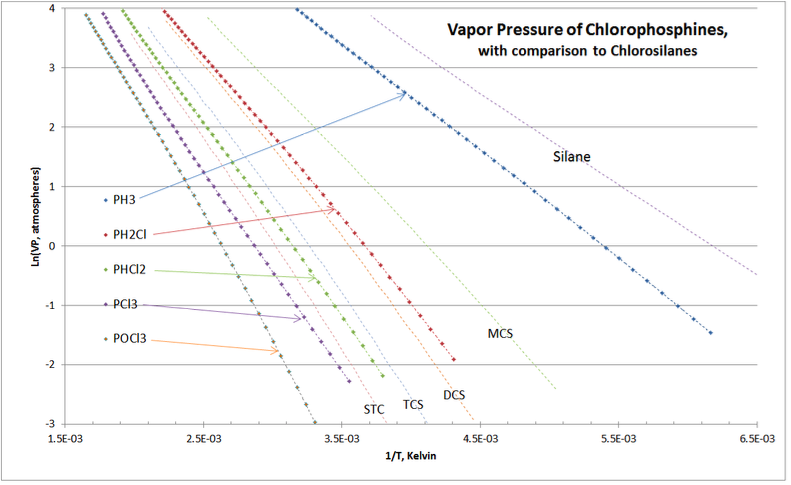
As expected, the chlorophosphine homologue’s VP curves “nest” around those of the chlorosilanes. There are no cross-overs of the curves, and the location of chlorophosphine vapor pressure curves lie exactly as they are experienced in commercial practice of chlorosilane purification distillation columns.

Since the math in Equation (\ref{4-3}) is somewhat involved, an example is provided with calculations.

Example: At 3.50 atmospheres pressure what is the boiling point of trichlorosilane (TCS)?

From Part III, Table 3-3, the pertinent property values for TCS are: T_c=479.15°K and P_c=41.15 atm. MW, T_b , V_c and Z_c are not needed for this example. From Part IV, the VP solution constants for TCS are: A=9.9796; B₀=1.1501; B₁=0.38395; B₂=-0.11827; B₃=0.063708; c=2.5687; n=5.7950; and k=0.0446.

As all advanced VP equations are, determining the TCS boiling point at 3.50 atmospheres is iterative; so it is nice to have a VP plot to get a good first guess. Using above Figure 4‑4, for

\ln (VP) =\ln (3.50) = 1.2528, it looks like 1/T= 2.89E-3 might be a good first guess => T=346°K; so first guess T_r=346/479.15 =0.7221. Plugging that first guess value of T_r into the T-S VP equation with the constants above:

\( \ln (P_{r})= A[B_{0}-T_{r}^{-1}-B_{1}\ln T_{r}+B_{2}T_{r}-(1/2)B_{3}T_{r}^2]+c[\frac{T_{r}^{n-1}-1}{n-1} +k(T_{r}^{-1}-1)] \nonumber\) yields a reduced VP value of P_r = 0.08273; so VP=0.08273*41.15 = 3.404 atm, which is just a bit less than the desired 3.50 atm. So T needs to increase a little from the 346°K initial first guess.

Re-doing the TCS VP equation with T= 347°K yields a VP of 3.50 atm (note: 347.05°K is the answer, if the solution is worked out to two decimal places of temperature). So the boiling temperature at 3.50 atmospheres is 347°K or 73.9°C.