
8: VLE Analysis Methods
- Page ID
- 8146

\( \newcommand{\vecs}[1]{\overset { \scriptstyle \rightharpoonup} {\mathbf{#1}} } \)
\( \newcommand{\vecd}[1]{\overset{-\!-\!\rightharpoonup}{\vphantom{a}\smash {#1}}} \)
\( \newcommand{\dsum}{\displaystyle\sum\limits} \)
\( \newcommand{\dint}{\displaystyle\int\limits} \)
\( \newcommand{\dlim}{\displaystyle\lim\limits} \)
\( \newcommand{\id}{\mathrm{id}}\) \( \newcommand{\Span}{\mathrm{span}}\)
( \newcommand{\kernel}{\mathrm{null}\,}\) \( \newcommand{\range}{\mathrm{range}\,}\)
\( \newcommand{\RealPart}{\mathrm{Re}}\) \( \newcommand{\ImaginaryPart}{\mathrm{Im}}\)
\( \newcommand{\Argument}{\mathrm{Arg}}\) \( \newcommand{\norm}[1]{\| #1 \|}\)
\( \newcommand{\inner}[2]{\langle #1, #2 \rangle}\)
\( \newcommand{\Span}{\mathrm{span}}\)
\( \newcommand{\id}{\mathrm{id}}\)
\( \newcommand{\Span}{\mathrm{span}}\)
\( \newcommand{\kernel}{\mathrm{null}\,}\)
\( \newcommand{\range}{\mathrm{range}\,}\)
\( \newcommand{\RealPart}{\mathrm{Re}}\)
\( \newcommand{\ImaginaryPart}{\mathrm{Im}}\)
\( \newcommand{\Argument}{\mathrm{Arg}}\)
\( \newcommand{\norm}[1]{\| #1 \|}\)
\( \newcommand{\inner}[2]{\langle #1, #2 \rangle}\)
\( \newcommand{\Span}{\mathrm{span}}\) \( \newcommand{\AA}{\unicode[.8,0]{x212B}}\)
\( \newcommand{\vectorA}[1]{\vec{#1}} % arrow\)
\( \newcommand{\vectorAt}[1]{\vec{\text{#1}}} % arrow\)
\( \newcommand{\vectorB}[1]{\overset { \scriptstyle \rightharpoonup} {\mathbf{#1}} } \)
\( \newcommand{\vectorC}[1]{\textbf{#1}} \)
\( \newcommand{\vectorD}[1]{\overrightarrow{#1}} \)
\( \newcommand{\vectorDt}[1]{\overrightarrow{\text{#1}}} \)
\( \newcommand{\vectE}[1]{\overset{-\!-\!\rightharpoonup}{\vphantom{a}\smash{\mathbf {#1}}}} \)
\( \newcommand{\vecs}[1]{\overset { \scriptstyle \rightharpoonup} {\mathbf{#1}} } \)
\(\newcommand{\longvect}{\overrightarrow}\)
\( \newcommand{\vecd}[1]{\overset{-\!-\!\rightharpoonup}{\vphantom{a}\smash {#1}}} \)
\(\newcommand{\avec}{\mathbf a}\) \(\newcommand{\bvec}{\mathbf b}\) \(\newcommand{\cvec}{\mathbf c}\) \(\newcommand{\dvec}{\mathbf d}\) \(\newcommand{\dtil}{\widetilde{\mathbf d}}\) \(\newcommand{\evec}{\mathbf e}\) \(\newcommand{\fvec}{\mathbf f}\) \(\newcommand{\nvec}{\mathbf n}\) \(\newcommand{\pvec}{\mathbf p}\) \(\newcommand{\qvec}{\mathbf q}\) \(\newcommand{\svec}{\mathbf s}\) \(\newcommand{\tvec}{\mathbf t}\) \(\newcommand{\uvec}{\mathbf u}\) \(\newcommand{\vvec}{\mathbf v}\) \(\newcommand{\wvec}{\mathbf w}\) \(\newcommand{\xvec}{\mathbf x}\) \(\newcommand{\yvec}{\mathbf y}\) \(\newcommand{\zvec}{\mathbf z}\) \(\newcommand{\rvec}{\mathbf r}\) \(\newcommand{\mvec}{\mathbf m}\) \(\newcommand{\zerovec}{\mathbf 0}\) \(\newcommand{\onevec}{\mathbf 1}\) \(\newcommand{\real}{\mathbb R}\) \(\newcommand{\twovec}[2]{\left[\begin{array}{r}#1 \\ #2 \end{array}\right]}\) \(\newcommand{\ctwovec}[2]{\left[\begin{array}{c}#1 \\ #2 \end{array}\right]}\) \(\newcommand{\threevec}[3]{\left[\begin{array}{r}#1 \\ #2 \\ #3 \end{array}\right]}\) \(\newcommand{\cthreevec}[3]{\left[\begin{array}{c}#1 \\ #2 \\ #3 \end{array}\right]}\) \(\newcommand{\fourvec}[4]{\left[\begin{array}{r}#1 \\ #2 \\ #3 \\ #4 \end{array}\right]}\) \(\newcommand{\cfourvec}[4]{\left[\begin{array}{c}#1 \\ #2 \\ #3 \\ #4 \end{array}\right]}\) \(\newcommand{\fivevec}[5]{\left[\begin{array}{r}#1 \\ #2 \\ #3 \\ #4 \\ #5 \\ \end{array}\right]}\) \(\newcommand{\cfivevec}[5]{\left[\begin{array}{c}#1 \\ #2 \\ #3 \\ #4 \\ #5 \\ \end{array}\right]}\) \(\newcommand{\mattwo}[4]{\left[\begin{array}{rr}#1 \amp #2 \\ #3 \amp #4 \\ \end{array}\right]}\) \(\newcommand{\laspan}[1]{\text{Span}\{#1\}}\) \(\newcommand{\bcal}{\cal B}\) \(\newcommand{\ccal}{\cal C}\) \(\newcommand{\scal}{\cal S}\) \(\newcommand{\wcal}{\cal W}\) \(\newcommand{\ecal}{\cal E}\) \(\newcommand{\coords}[2]{\left\{#1\right\}_{#2}}\) \(\newcommand{\gray}[1]{\color{gray}{#1}}\) \(\newcommand{\lgray}[1]{\color{lightgray}{#1}}\) \(\newcommand{\rank}{\operatorname{rank}}\) \(\newcommand{\row}{\text{Row}}\) \(\newcommand{\col}{\text{Col}}\) \(\renewcommand{\row}{\text{Row}}\) \(\newcommand{\nul}{\text{Nul}}\) \(\newcommand{\var}{\text{Var}}\) \(\newcommand{\corr}{\text{corr}}\) \(\newcommand{\len}[1]{\left|#1\right|}\) \(\newcommand{\bbar}{\overline{\bvec}}\) \(\newcommand{\bhat}{\widehat{\bvec}}\) \(\newcommand{\bperp}{\bvec^\perp}\) \(\newcommand{\xhat}{\widehat{\xvec}}\) \(\newcommand{\vhat}{\widehat{\vvec}}\) \(\newcommand{\uhat}{\widehat{\uvec}}\) \(\newcommand{\what}{\widehat{\wvec}}\) \(\newcommand{\Sighat}{\widehat{\Sigma}}\) \(\newcommand{\lt}{<}\) \(\newcommand{\gt}{>}\) \(\newcommand{\amp}{&}\) \(\definecolor{fillinmathshade}{gray}{0.9}\)Distillation Science (a blend of Chemistry and Chemical Engineering)
This is Part VIII, VLE Analysis Methods of a ten-part series of technical articles on Distillation Science, as is currently practiced on an industrial level. See also Part I, Overview for introductory comments, the scope of the article series, and nomenclature.
Part VIII, VLE Analysis Methods recommends methodology used when data-collecting the Liquid Activity Coefficients of binary systems (see Part VII). This article also deals with validation, especially when data collection is done on reactive fluids like chlorosilanes which can disproportionate or dimerize during study.
This article uses the information of Parts III through VII.
In Part VII a correlation technique was given for estimating Liquid Activity Coefficients. As mentioned in the previous article it is common to collect such vapor-liquid equilibria (VLE) data in the lab, at conditions close to ambient pressure. Yet many industrial applications frequently need to use VLE results at higher process pressure/temperatures or different compositions. To avoid notation confusion between the liquid activity coefficient (\(\gamma_{i} \nonumber\)) and the vapor mole fraction (Yi), the mole fractions X and Y are shown as bolded.
Recall from Parts VI and VII that fugacity coefficients (\(\phi_{i}^V\nonumber\)& \(\phi_{i}^L\nonumber\)) are functions of temperature and pressure. However, Liquid Activity Coefficient s ( \(\gamma_{i} \nonumber\) ) are functions of only temperature and mole fraction. In an experimental situation, the calculated values of \(\gamma_{i} \nonumber\) (from the values of Yi and Xi = vapor-phase mole fraction and liquid-phase mole fraction) are easiest to correlate when system temperature is held constant, and system pressure is allowed to vary. Stated otherwise, PXY data @ constant T is far easier to collect and correlate than TXY @ constant P. However, in commercial applications the distillation column is typically controlled at constant pressure. So a common industrial communication error is to request the lab to collect VLE data as TXY@P, but instead get PXY@T instead. There is a way to convert one data set to the other relationship, but it is somewhat awkward and requires choosing activity coefficient model.
In Figure 7-1 of Part VII, the expected profile of \(\gamma \nonumber\) vs X @ constant T is shown, and in Figure 7-2 of Part VII the expected profile of \(\gamma \nonumber\) vs T @ constant X is shown, at the X=0 and X=1 axes. The reason for generating Liquid Activity Coefficients experimentally is normally to use the lab results for distillation column design, with the confidence that \(\gamma \nonumber\) can be accurately known at any value of X or T, so as to establish the Y/X relationship up and down the column design. Using the principles of Parts VI and VII, these problems can be resolved.
Having established the experimental protocol, it is necessary to consider the impact of data collection equipment on the fluids being analyzed and to validate the quality of the sample fluids. For reactive fluids such as chlorosilanes, that means using pressure-capable glassware is the best choice (or nickel-lined steel as a second choice), since some of the alloying elements of stainless steel will slowly catalyze disproportionation reactions, which alter the sample compositions.
Also, it is important to validate the purity of the fluid samples, as opposed to blindly accepting the analysis of any accompanying supplier information. Again, with chlorosilanes (as typical of reactive fluids), the shipping container can catalyze side reactions (i.e., the supplier’s COA was perhaps accurate when the sample was loaded into the container, but purity degraded during shipment). It is common for 99.99% pure TCS samples (under argon inerting) from reputable suppliers to end up having several percent DCS and several percent STC, along with a few tenths percent hexachlorodisilane and a few tenths percent hydrogen gas, when used just a few weeks later. A good practice before loading sample fluids into the lab equipment is to double-distill samples (discarding the “lights” and “heavies” fractions, and assuring that only the “heart’s cut” fraction is used: whose boiling pressure is identical to the expected pure component vapor pressure).
With the above precautions, data is collected at 15-20 (or more) X,Y points, with some duplicates later in the run to establish experimental analysis accuracy and confirm the absence of systemic error (such as contamination). At least two pairs of data points should be collected close to X= zero and X= unity. To help confirm temperature dependency of activity coefficients, at least three sets of data (each at a different constant temperature or pressure) should be collected.
After data collection, the lab work is suspended, but then "number-crunching" is needed to confirm the data’s validity before reporting or using the results. If data validity is not confirmed, the error must be found and lab work repeated. First, plot out the data set and check that both the P-X curve and P-Y curve , or T-X curve and T-Y curve show an identical intersection, at both zero and unity mole fraction axes; and that the axis intersections are exactly representative of each pure-component’s known vapor pressure. If the X and Y curves do not intersect at the correct value on each axis, there is some systematic error in the data set that must be resolved before any more evaluation work is done. A corrupted dataset is likely to be of only minimal value in establishing activity coefficients; and is more often a reason to toss it all out and re-do the work, after the systemic error is resolved.
Using an algebraic modification of previous Equation 6-4, activity coefficients, the \(\gamma_{i} \nonumber\) i are calculated for each P-X and P-Y data point.
\[\gamma_{i} =(\phi_{i}^V/\phi_{i}^L) \times (Y_{i} \times \pi)/(VP_{i} \times X_{i}) \label{8-1} \]
where \(\pi \nonumber\) is the total pressure, \(VP_{i} \nonumber\) is the vapor pressure of the ith component, and \((\phi_{i}^V/\phi_{i}^L) \nonumber\) is the vapor/liquid fugacity ratio of that component.
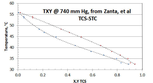
In Figure 8-1 the twelve-point TXY/P data set of Zanta et al, from Chemicky Prumysl (Czech Chemical Industry) is shown, using a spreadsheet plot. The researchers did collect a few data points near the STC axis (i.e., TCS= zero). However it would have been preferable to have a few more collected close to the other (i.e., TCS= unity) axis; and to have that all data reported with more precision. The researchers chose to collect data at a constant pressure of 740 mm Hg (as opposed to the more preferable PXY/T method that avoids the need for adjustment of calculated Liquid Activity Coefficient \(\gamma \nonumber\) for changing temperature), for reasons of their lab equipment and simplifying their procedure; and to only collect one TXY/P data set.
If only the raw data is considered, it would appear that the T-X and T-Y curves might not mutually intersect at the STC axis, or that the intersection is higher than the expected 56.2°C temperature representative of STC vaporization @ 740 mm Hg. The reason is that individual data point precision is low in the region of the STC axis.
However, with data-smoothing and extrapolation of the T-X and T-Y curves via some spreadsheet curve-fitting, the two curves appear to quite likely both intersect the STC axis near the expected 56.2°C temperature. At the TCS axis however, curve-fitting the T-X and T-Y data appears to both result in their intersection on the TCS axis at 30.0°C, as opposed to the expected 32.3°C for pure TCS. The most likely explanation for this data set discrepancy is that the TCS sample supplied was either a disproportionated mix of DCS/TCS/STC as-received, and/or the fluids in the equipment disproportionated as a result of the equipment materials of construction. A TCS axis temperature of 30.0°C is representative of a 5% DCS/95% TCS liquid mixture. Surprisingly, the researchers’ analytical procedure did not pick up the DCS peak, which would have revealed the sample corruption ( but that is a common error using that the researcher’s type of analyzer).
Now that the data set has been discredited, it remains to be seen what - if any- useful information can be extracted. Other than demonstrating technique, there is little use in reducing the data that is high in “bad TCS” to get the \(\gamma \nonumber\) asymptote intersecting the TCS axis. That is because the XTCS* mole fractions are changing along the STC activity coefficient curve (about a high 1:19 ratio of DCS/TCS, dropping in ratio to very little DCS in the ternary mixture, close to 56.2°C at the STC axis). It would be impossible to guess what property values are best to use for fugacity coefficients, given a “wild-card” DCS content). The data closest to intersecting the STC axis could be interpolated to make up a few “pseudo-points” close to XTCS=0, in order to get a rough value of the TCS \(\gamma \nonumber\) asymptote (based on the assumption that there is little DCS in the ternary mix at that point). However, even small amounts of DCS near the XTCS=0 area could be expected to exert a significant Liquid Activity Coefficient effect, and the fugacity values might be somewhat in error by assuming only the property values of TCS.
However, to illustrate the data reduction technique for TXY/P data (as opposed to the preferred PXY/T form), a few “pseudo-points” are evaluated near the axis.
Using a fourth order curve-fit, with the STC axis temperature set to 56.20°C, the T-X and T-Y curve-fit equations are, respectively, via spreadsheet curve-fitting functions:
T-X \(T=18.949x^4-64.825x^3+75.709x^2-56.044x+ 56.20 \nonumber\)
T-Y \(T=-22.243y^4+33.158y^3-18.028y^2-19.075y+ 56.20 \nonumber\)
From those two curve-fits, the following “pseudo-points” are calculated, by solving the quartic equations for T-X and T-Y:
|
P, mm Hg |
T, °C |
XTCS* |
\(\gamma \nonumber\) TCS* |
|---|---|---|---|
|
740 |
56.2 |
0.0000 |
0.0000 |
|
740 |
55.0 |
0.00359 |
0.0104 |
|
740 |
54.0 |
0.0415 |
0.1065 |
|
740 |
53.0 |
0.0620 |
0.1515 |
In Table 8-1, XTCS* and YTCS* are subscripted as "TCS*" to denote that while TCS properties are used for vapor pressure and fugacity estimation, the more volatile fluid is really a DCS/TCS mix. The data-point at X, Y = 0.0000, 0.0000 is given just to show the STC axis intersection, but cannot be used to calculate the \(\gamma \nonumber\) asymptote since that would result in “division by zero” in Equation 7-1.
Using the properties of TCS, the values for VP, øL and øv are calculated as per Parts IV, V, and VI, and the results shown in Table 8-2 for calculated \(\gamma \nonumber\) TCS* at 740mm Hg (for each “pseudo-point” temperature).
|
P, mm Hg |
T, °C |
VPTCS* |
øL |
øv |
\(\gamma \nonumber\) TCS* |
|---|---|---|---|---|---|
|
740 |
56.2 |
2.130 |
0.9983 |
1.0321 |
to be determined |
|
740 |
55.0 |
2.055 |
0.9984 |
1.0316 |
1.418 |
|
740 |
54.0 |
1.994 |
0.9984 |
1.0311 |
1.294 |
|
740 |
53.0 |
1.934 |
0.9984 |
1.0307 |
1.270 |
The calculated values for \(\gamma \nonumber\) TCS* in Table 8-2 are based on the X,Y “pseudo-points” of Table 8-1 and using Equation (\ref{8-1}) above, to demonstrate the methodology of experimental data reduction. The trending on fugacity coefficients and activity coefficient is correct: øL values increase toward unity as XTCS* increases toward unity; øv values decrease toward unity as XTCS* increases toward unity; \(\gamma \nonumber\) TCS* values decrease toward unity as XTCS* increases toward unity.
The asymptote at the STC axis is determined by extrapolating value of \(\gamma \nonumber\) TCS* from the three “pseudo-points”. (That curve would have a different slope with respect to composition if it were TXY/P data, since temperature is changing as well as XTCS* in Table 7-2.) This technique identifies the \(\gamma \nonumber\) TCS* asymptote as 1.437 (the average value of \(\gamma \nonumber\) TCS* obtained by extrapolating curve-fits of \(\gamma \nonumber\) TCS* vs XTCS* to a zero value of XTCS*, and \(\gamma \nonumber\) TCS* vs YTCS* to a zero value of XTCS*). Compared to other researcher’s data, the calculated asymptote has a high value. It also seems high per expectation from Equation 7-3 from Part VII, which would indicate a value closer to 1.21 @ 56.2°C, or 1.23 @ 32.3°C (the expected TCS boiling point at 740 mm Hg). Possibly there is error from the DCS content, which would tend to make the calculated \(\gamma \nonumber\) TCS* values high by increasing the non-STC mole fraction in the vapor. The curve-fitting technique could be “off” since there was low precision in the two data pairs close to the XTCS* =0 axis.
This demonstrates that there is simply no good way to “fix” data that has systematic error in it: virtually all texts suggest that when corrupted data is encountered, it is pointless to continue with data analysis. In addition to determining reasonable asymptotic values at either axis, Reid, Prausnitz, and Sherwood suggest in “The Properties of Gases and Liquids”, that all \(\gamma \nonumber\) calculated values be first adjusted to a common temperature basis (using the approximation of \(Ln(\gamma) \times = constant \nonumber\)), then use the Gibbs-Duhem Law to establish thermodynamic consistency. While technically the best way to validate data for consistency, it requires a significant amount of high-quality data, and is suggested only if advanced Liquid Activity Coefficient models are to be considered (e.g., NRTL or UNIQUAC). For Van Laar, Margules, Wilson or similar two-constant models, 15-20 data points should be sufficient.
It is always better to have fewer data points, but have the dataset internally consistent, rather than a large number of possibly corrupted data points.
This article suggests using the Van Laar model for activity coefficients based on reasonable results with data analysis on chlorosilanes, and the success in predicting the Van Laar constants via Equation 7-3 in Part VII. However, the reader may want to explore other models for a better fit to experimental data, after such data has been validated. In “The Properties of Gases and Liquids”, the authors give an exhaustive list of other activity coefficient models to consider, with some notes on “pro & con”.