12: Appendix A- Taylor Series Expansions
- Page ID
- 18038

\( \newcommand{\vecs}[1]{\overset { \scriptstyle \rightharpoonup} {\mathbf{#1}} } \)
\( \newcommand{\vecd}[1]{\overset{-\!-\!\rightharpoonup}{\vphantom{a}\smash {#1}}} \)
\( \newcommand{\id}{\mathrm{id}}\) \( \newcommand{\Span}{\mathrm{span}}\)
( \newcommand{\kernel}{\mathrm{null}\,}\) \( \newcommand{\range}{\mathrm{range}\,}\)
\( \newcommand{\RealPart}{\mathrm{Re}}\) \( \newcommand{\ImaginaryPart}{\mathrm{Im}}\)
\( \newcommand{\Argument}{\mathrm{Arg}}\) \( \newcommand{\norm}[1]{\| #1 \|}\)
\( \newcommand{\inner}[2]{\langle #1, #2 \rangle}\)
\( \newcommand{\Span}{\mathrm{span}}\)
\( \newcommand{\id}{\mathrm{id}}\)
\( \newcommand{\Span}{\mathrm{span}}\)
\( \newcommand{\kernel}{\mathrm{null}\,}\)
\( \newcommand{\range}{\mathrm{range}\,}\)
\( \newcommand{\RealPart}{\mathrm{Re}}\)
\( \newcommand{\ImaginaryPart}{\mathrm{Im}}\)
\( \newcommand{\Argument}{\mathrm{Arg}}\)
\( \newcommand{\norm}[1]{\| #1 \|}\)
\( \newcommand{\inner}[2]{\langle #1, #2 \rangle}\)
\( \newcommand{\Span}{\mathrm{span}}\) \( \newcommand{\AA}{\unicode[.8,0]{x212B}}\)
\( \newcommand{\vectorA}[1]{\vec{#1}} % arrow\)
\( \newcommand{\vectorAt}[1]{\vec{\text{#1}}} % arrow\)
\( \newcommand{\vectorB}[1]{\overset { \scriptstyle \rightharpoonup} {\mathbf{#1}} } \)
\( \newcommand{\vectorC}[1]{\textbf{#1}} \)
\( \newcommand{\vectorD}[1]{\overrightarrow{#1}} \)
\( \newcommand{\vectorDt}[1]{\overrightarrow{\text{#1}}} \)
\( \newcommand{\vectE}[1]{\overset{-\!-\!\rightharpoonup}{\vphantom{a}\smash{\mathbf {#1}}}} \)
\( \newcommand{\vecs}[1]{\overset { \scriptstyle \rightharpoonup} {\mathbf{#1}} } \)
\( \newcommand{\vecd}[1]{\overset{-\!-\!\rightharpoonup}{\vphantom{a}\smash {#1}}} \)
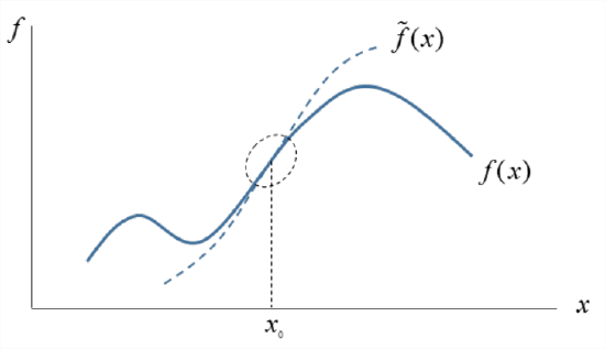
\(\newcommand{\avec}{\mathbf a}\) \(\newcommand{\bvec}{\mathbf b}\) \(\newcommand{\cvec}{\mathbf c}\) \(\newcommand{\dvec}{\mathbf d}\) \(\newcommand{\dtil}{\widetilde{\mathbf d}}\) \(\newcommand{\evec}{\mathbf e}\) \(\newcommand{\fvec}{\mathbf f}\) \(\newcommand{\nvec}{\mathbf n}\) \(\newcommand{\pvec}{\mathbf p}\) \(\newcommand{\qvec}{\mathbf q}\) \(\newcommand{\svec}{\mathbf s}\) \(\newcommand{\tvec}{\mathbf t}\) \(\newcommand{\uvec}{\mathbf u}\) \(\newcommand{\vvec}{\mathbf v}\) \(\newcommand{\wvec}{\mathbf w}\) \(\newcommand{\xvec}{\mathbf x}\) \(\newcommand{\yvec}{\mathbf y}\) \(\newcommand{\zvec}{\mathbf z}\) \(\newcommand{\rvec}{\mathbf r}\) \(\newcommand{\mvec}{\mathbf m}\) \(\newcommand{\zerovec}{\mathbf 0}\) \(\newcommand{\onevec}{\mathbf 1}\) \(\newcommand{\real}{\mathbb R}\) \(\newcommand{\twovec}[2]{\left[\begin{array}{r}#1 \\ #2 \end{array}\right]}\) \(\newcommand{\ctwovec}[2]{\left[\begin{array}{c}#1 \\ #2 \end{array}\right]}\) \(\newcommand{\threevec}[3]{\left[\begin{array}{r}#1 \\ #2 \\ #3 \end{array}\right]}\) \(\newcommand{\cthreevec}[3]{\left[\begin{array}{c}#1 \\ #2 \\ #3 \end{array}\right]}\) \(\newcommand{\fourvec}[4]{\left[\begin{array}{r}#1 \\ #2 \\ #3 \\ #4 \end{array}\right]}\) \(\newcommand{\cfourvec}[4]{\left[\begin{array}{c}#1 \\ #2 \\ #3 \\ #4 \end{array}\right]}\) \(\newcommand{\fivevec}[5]{\left[\begin{array}{r}#1 \\ #2 \\ #3 \\ #4 \\ #5 \\ \end{array}\right]}\) \(\newcommand{\cfivevec}[5]{\left[\begin{array}{c}#1 \\ #2 \\ #3 \\ #4 \\ #5 \\ \end{array}\right]}\) \(\newcommand{\mattwo}[4]{\left[\begin{array}{rr}#1 \amp #2 \\ #3 \amp #4 \\ \end{array}\right]}\) \(\newcommand{\laspan}[1]{\text{Span}\{#1\}}\) \(\newcommand{\bcal}{\cal B}\) \(\newcommand{\ccal}{\cal C}\) \(\newcommand{\scal}{\cal S}\) \(\newcommand{\wcal}{\cal W}\) \(\newcommand{\ecal}{\cal E}\) \(\newcommand{\coords}[2]{\left\{#1\right\}_{#2}}\) \(\newcommand{\gray}[1]{\color{gray}{#1}}\) \(\newcommand{\lgray}[1]{\color{lightgray}{#1}}\) \(\newcommand{\rank}{\operatorname{rank}}\) \(\newcommand{\row}{\text{Row}}\) \(\newcommand{\col}{\text{Col}}\) \(\renewcommand{\row}{\text{Row}}\) \(\newcommand{\nul}{\text{Nul}}\) \(\newcommand{\var}{\text{Var}}\) \(\newcommand{\corr}{\text{corr}}\) \(\newcommand{\len}[1]{\left|#1\right|}\) \(\newcommand{\bbar}{\overline{\bvec}}\) \(\newcommand{\bhat}{\widehat{\bvec}}\) \(\newcommand{\bperp}{\bvec^\perp}\) \(\newcommand{\xhat}{\widehat{\xvec}}\) \(\newcommand{\vhat}{\widehat{\vvec}}\) \(\newcommand{\uhat}{\widehat{\uvec}}\) \(\newcommand{\what}{\widehat{\wvec}}\) \(\newcommand{\Sighat}{\widehat{\Sigma}}\) \(\newcommand{\lt}{<}\) \(\newcommand{\gt}{>}\) \(\newcommand{\amp}{&}\) \(\definecolor{fillinmathshade}{gray}{0.9}\)Taylor’s theorem (which we will not prove here) gives us a way to take a complicated function \(f(x)\) and approximate it by a simpler function \(\tilde{f}(x)\). The price of this simplification is that \(\tilde{f} \approx f\) only in a small region surrounding some point \(x = x_0\) (Figure \(\PageIndex{1}\)).
The formula is:
\[\tilde{f}(x)=f\left(x_{0}\right)+f^{\prime}\left(x_{0}\right)\left(x-x_{0}\right)+\frac{1}{2} f^{\prime \prime}\left(x_{0}\right)\left(x-x_{0}\right)^{2}+\frac{1}{6} f^{\prime \prime \prime}\left(x_{0}\right)\left(x-x_{0}\right)^{3}+\dots\label{eqn:1} \]
The sequence goes on forever, but we typically only use the first few terms. To apply (1), we choose a point \(x_0\) where we need the approximation to be accurate. We then compute the derivatives at that point, \(f^\prime(x_0)\, \(f^{\prime\prime} (x_0)\), \(f^{\prime\prime\prime} (x_0)\), etc., for as far as we want to take it. For accuracy, use a lot of terms; for simplicity, use only a few.
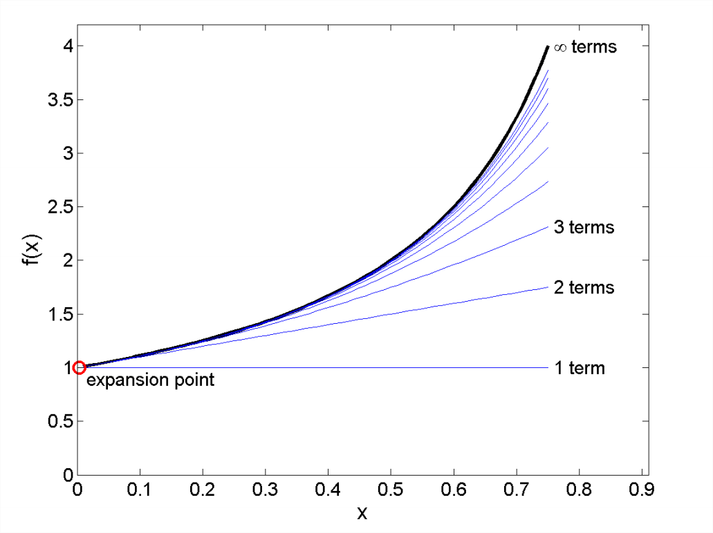
For example, if
\[f(x)=(1-x)^{-1} \nonumber \]
and we choose \(x_0\) = 0, then the Taylor series is just the well-known expression
\[\tilde{f}(x)=1+x+x^2+x^3+\dots. \nonumber \]
Figure A.2 shows the expansion with successively larger numbers of terms retained. Near x0, good accuracy can be achieved with only a few terms. The further you get from x0, the more terms must be retained for a given level of accuracy.
The real benefit of Taylor series is evident when working with more complicated functions. For example, \(f(x) = \sin(\tan(x))\) can be approximated by \(\tilde{f}\) = \(x\) for \(x\) close to zero.
Note that the first - order terms in Equation \(\ref{eqn:1}\):
\[\tilde{f}(x)=f(x_0)+f^\prime(x_0)(x-x_0), \nonumber \]
give a valid approximation of \(f(x)\) in the limit \(x \rightarrow x_0\), and can be rearranged to form the familiar definition of the first derivative:
\[f^\prime(x_0)=\lim{x\to x_0}\frac{f(x)-f(x_0)}{x-x_0} \nonumber \]
The Taylor series expansion technique can be generalized for use with multivariate functions. Suppose that \(f = f(\vec{x})\), where \(\vec{x} = (x, y)\). Then
\[\tilde{f}(\vec{x})=f(\vec{x_0})+f_x(\vec{x_0})\delta x+ f_y(\vec{x_0})\delta y + \frac{1}{2} f_{xx}(\vec{x_0})\delta x^2 + f_{xy}(\vec{x_0})\delta_x\delta_y+\frac{1}{2}f_{yy}(\vec{x_0})\delta_{y^2}+\dots,\label{eqn:2} \]
where \(\delta_x=x-x_0\), \(\delta_y=y-y_0\) and subscripts denote partial derivatives. Note that the first - order terms in Equation \(\ref{eqn:2}\) can be written using the directional derivative:
\[f(\vec{x})=f(\vec{x_0})+\vec{\nabla}f(\vec{x_0})\cdot\delta \vec{x}. \nonumber \]
You will notice that \(\tilde{f}\) has been replaced by \(f\); this is valid in the limit \(\vec{x} \rightarrow \vec{x_0}\), or \(\delta \vec{x} \rightarrow 0\).