
11: Exercises
- Page ID
- 18049

\( \newcommand{\vecs}[1]{\overset { \scriptstyle \rightharpoonup} {\mathbf{#1}} } \)
\( \newcommand{\vecd}[1]{\overset{-\!-\!\rightharpoonup}{\vphantom{a}\smash {#1}}} \)
\( \newcommand{\dsum}{\displaystyle\sum\limits} \)
\( \newcommand{\dint}{\displaystyle\int\limits} \)
\( \newcommand{\dlim}{\displaystyle\lim\limits} \)
\( \newcommand{\id}{\mathrm{id}}\) \( \newcommand{\Span}{\mathrm{span}}\)
( \newcommand{\kernel}{\mathrm{null}\,}\) \( \newcommand{\range}{\mathrm{range}\,}\)
\( \newcommand{\RealPart}{\mathrm{Re}}\) \( \newcommand{\ImaginaryPart}{\mathrm{Im}}\)
\( \newcommand{\Argument}{\mathrm{Arg}}\) \( \newcommand{\norm}[1]{\| #1 \|}\)
\( \newcommand{\inner}[2]{\langle #1, #2 \rangle}\)
\( \newcommand{\Span}{\mathrm{span}}\)
\( \newcommand{\id}{\mathrm{id}}\)
\( \newcommand{\Span}{\mathrm{span}}\)
\( \newcommand{\kernel}{\mathrm{null}\,}\)
\( \newcommand{\range}{\mathrm{range}\,}\)
\( \newcommand{\RealPart}{\mathrm{Re}}\)
\( \newcommand{\ImaginaryPart}{\mathrm{Im}}\)
\( \newcommand{\Argument}{\mathrm{Arg}}\)
\( \newcommand{\norm}[1]{\| #1 \|}\)
\( \newcommand{\inner}[2]{\langle #1, #2 \rangle}\)
\( \newcommand{\Span}{\mathrm{span}}\) \( \newcommand{\AA}{\unicode[.8,0]{x212B}}\)
\( \newcommand{\vectorA}[1]{\vec{#1}} % arrow\)
\( \newcommand{\vectorAt}[1]{\vec{\text{#1}}} % arrow\)
\( \newcommand{\vectorB}[1]{\overset { \scriptstyle \rightharpoonup} {\mathbf{#1}} } \)
\( \newcommand{\vectorC}[1]{\textbf{#1}} \)
\( \newcommand{\vectorD}[1]{\overrightarrow{#1}} \)
\( \newcommand{\vectorDt}[1]{\overrightarrow{\text{#1}}} \)
\( \newcommand{\vectE}[1]{\overset{-\!-\!\rightharpoonup}{\vphantom{a}\smash{\mathbf {#1}}}} \)
\( \newcommand{\vecs}[1]{\overset { \scriptstyle \rightharpoonup} {\mathbf{#1}} } \)
\( \newcommand{\vecd}[1]{\overset{-\!-\!\rightharpoonup}{\vphantom{a}\smash {#1}}} \)
\(\newcommand{\avec}{\mathbf a}\) \(\newcommand{\bvec}{\mathbf b}\) \(\newcommand{\cvec}{\mathbf c}\) \(\newcommand{\dvec}{\mathbf d}\) \(\newcommand{\dtil}{\widetilde{\mathbf d}}\) \(\newcommand{\evec}{\mathbf e}\) \(\newcommand{\fvec}{\mathbf f}\) \(\newcommand{\nvec}{\mathbf n}\) \(\newcommand{\pvec}{\mathbf p}\) \(\newcommand{\qvec}{\mathbf q}\) \(\newcommand{\svec}{\mathbf s}\) \(\newcommand{\tvec}{\mathbf t}\) \(\newcommand{\uvec}{\mathbf u}\) \(\newcommand{\vvec}{\mathbf v}\) \(\newcommand{\wvec}{\mathbf w}\) \(\newcommand{\xvec}{\mathbf x}\) \(\newcommand{\yvec}{\mathbf y}\) \(\newcommand{\zvec}{\mathbf z}\) \(\newcommand{\rvec}{\mathbf r}\) \(\newcommand{\mvec}{\mathbf m}\) \(\newcommand{\zerovec}{\mathbf 0}\) \(\newcommand{\onevec}{\mathbf 1}\) \(\newcommand{\real}{\mathbb R}\) \(\newcommand{\twovec}[2]{\left[\begin{array}{r}#1 \\ #2 \end{array}\right]}\) \(\newcommand{\ctwovec}[2]{\left[\begin{array}{c}#1 \\ #2 \end{array}\right]}\) \(\newcommand{\threevec}[3]{\left[\begin{array}{r}#1 \\ #2 \\ #3 \end{array}\right]}\) \(\newcommand{\cthreevec}[3]{\left[\begin{array}{c}#1 \\ #2 \\ #3 \end{array}\right]}\) \(\newcommand{\fourvec}[4]{\left[\begin{array}{r}#1 \\ #2 \\ #3 \\ #4 \end{array}\right]}\) \(\newcommand{\cfourvec}[4]{\left[\begin{array}{c}#1 \\ #2 \\ #3 \\ #4 \end{array}\right]}\) \(\newcommand{\fivevec}[5]{\left[\begin{array}{r}#1 \\ #2 \\ #3 \\ #4 \\ #5 \\ \end{array}\right]}\) \(\newcommand{\cfivevec}[5]{\left[\begin{array}{c}#1 \\ #2 \\ #3 \\ #4 \\ #5 \\ \end{array}\right]}\) \(\newcommand{\mattwo}[4]{\left[\begin{array}{rr}#1 \amp #2 \\ #3 \amp #4 \\ \end{array}\right]}\) \(\newcommand{\laspan}[1]{\text{Span}\{#1\}}\) \(\newcommand{\bcal}{\cal B}\) \(\newcommand{\ccal}{\cal C}\) \(\newcommand{\scal}{\cal S}\) \(\newcommand{\wcal}{\cal W}\) \(\newcommand{\ecal}{\cal E}\) \(\newcommand{\coords}[2]{\left\{#1\right\}_{#2}}\) \(\newcommand{\gray}[1]{\color{gray}{#1}}\) \(\newcommand{\lgray}[1]{\color{lightgray}{#1}}\) \(\newcommand{\rank}{\operatorname{rank}}\) \(\newcommand{\row}{\text{Row}}\) \(\newcommand{\col}{\text{Col}}\) \(\renewcommand{\row}{\text{Row}}\) \(\newcommand{\nul}{\text{Nul}}\) \(\newcommand{\var}{\text{Var}}\) \(\newcommand{\corr}{\text{corr}}\) \(\newcommand{\len}[1]{\left|#1\right|}\) \(\newcommand{\bbar}{\overline{\bvec}}\) \(\newcommand{\bhat}{\widehat{\bvec}}\) \(\newcommand{\bperp}{\bvec^\perp}\) \(\newcommand{\xhat}{\widehat{\xvec}}\) \(\newcommand{\vhat}{\widehat{\vvec}}\) \(\newcommand{\uhat}{\widehat{\uvec}}\) \(\newcommand{\what}{\widehat{\wvec}}\) \(\newcommand{\Sighat}{\widehat{\Sigma}}\) \(\newcommand{\lt}{<}\) \(\newcommand{\gt}{>}\) \(\newcommand{\amp}{&}\) \(\definecolor{fillinmathshade}{gray}{0.9}\)All matrices are 3\(\times\)3 and all vectors are 3-vectors, unless otherwise specified.
- Combining vectors Let \[\vec{u}=\left[\begin{array}{l}
0 \\
1 \\
2
\end{array}\right] ; \quad \vec{v}=\left[\begin{array}{l}
1 \\
2 \\
3
\end{array}\right] \nonumber \] Compute the following:- \(\vec{u}\cdot\vec{v}\)
- \(|\vec{u}|\)
- \(|\vec{v}|\)
- \(\theta\)
- component of \(\vec{u}\) in the direction of \(\vec{v}\)
- component of \(\vec{v}\) in the direction of \(\vec{u}\)
- Self-consistency of free indices 1 In which of the following equations are the free indices consistent?
- \(A_{ij}B_j=\Gamma_i\)
- \(A_{ij}B_i=\Gamma_i\)
- \(A_{ij}B_j=\Gamma_i\)
- Matrix multiplication Which of the following expressions are equivalent to \(A_{ij}B_{jk}\)?
- \(A_{im}B_{mk}\)
- \(A^T_{mi}B_{mk}\)
- \(B_{jk}A_{ij}\)
- Self-consistency of free indices 2 Fill in the indices on Γ to make the equation self - consistent:
- \(A_{ij}B_{j}=\Gamma_?\)
- \(A_{kj}B_{j}=\Gamma_?\)
- \(A_{ik}B_k=\Gamma_?\)
- \(A_{iq}B_q=\Gamma_?\)
- \(A_{ij}B_{jk}=\Gamma_?\)
- \(A_{ik}B_{kj}=\Gamma_?\)
- \(A_{lm}B_{ma}=\Gamma_?\)
- \(A_{ij}B_{kj}C_{kl}=\Gamma_?\)
- Using the identity matrix Simplify the following by summing over the dummy indices. Assume that vectors have 3 elements and matrices are 3\(\times\)3.
- \(\delta_{3k}p_k\)
- \(\delta_{3i}\delta_{ij}\)
- \(\delta_{i2}\delta_{i2}\)
- \(\delta_{ij}\delta_{ij}\)
- \(\delta_{i2}\delta_{ik}\delta_{3k}\)
- \(\delta_{ij}v_iv_j\)
- Vector and matrix properties For each statement on the left, choose the appropriate statement from the list on the right.
-
\(u_iv_i=0\) \(\underset{\sim}{A}\) is an orthogonal matrix. \(A_{pq}B_{qr}=\delta_{pr}\) \(\vec{u}\) is an eigenvector of \(\underset{\sim}{A}\). \(A_{i j}+A_{j i}=0\) \(\underset{\sim}{B}\) is the inverse of \(\underset{\sim}{A}\). \{u_{i} v_{i}=\pm|\vec{u}||\vec{v}|\) \(\vec{u}\) and \(\vec{v}\) are orthogonal vectors. \(|\vec{v}|=1\) \(\underset{\sim}{A}\) is a symmetric matrix. \(A_{i j}^{T} A_{j k}=\delta_{i k}\) \(\vec{v}\) is a unit vector. \(\underset{\sim}{A}\) is an antisymmetric matrix. \(\vec{u}\) is parallel to \(\vec{v}\)
-
- Hyperbolic functions review The hyperbolic sine and cosine functions are defined as: \[\sinh x=\frac{e^{x}-e^{-x}}{2} ; \quad \cosh x=\frac{e^{x}+e^{-x}}{2} \nonumber \]
- Show that \[\frac{d}{d x} \sinh x=\cosh x ; \quad \frac{d}{d x} \cosh x=\sinh x \cdot \quad \frac{d^{2}}{d x^{2}} \sinh x=\sinh x. \nonumber \]
- Calculate the Taylor series expansions about \(x\) = 0 of \(f(x)\) = \(\sinh x\) and \(f(x)\) = \(\cosh x\) up to (and including) the term proportional to \(x^2\). [See Appendix A if you need a refresher on Taylor series.]
- Sketch the \(\sinh\) and \(\cosh\) functions.
- The hyperbolic tangent function is \[\tanh x=\frac{\sinh x}{\cosh x} \nonumber \] Using your results from (a) and (b) above, show that \(\tanh x \simeq x\) for \(x\) close to zero.
- Determine the limiting values of \(\tanh x\) as \(x \rightarrow \inf\) and as \(x \rightarrow −\inf\). (Hint: start by writing \(tanh x\) in terms of \(e^x\) and \(e^{−x}\).)
- Sketch the \(\tanh\) function.
- Matrix transformations 1 For each matrix, compute the determinant and describe in words the effect the matrix has on a general column vector \(\vec{v}\). Is the effect reversible?
- \[\left[\begin{array}{lll}
3 & 0 & 0 \\
0 & 3 & 0 \\
0 & 0 & 3
\end{array}\right] \nonumber \] - \[\left[\begin{array}{lll}
0 & 0 & 0 \\
0 & 1 & 0 \\
0 & 0 & 1
\end{array}\right] \nonumber \] - \[\left[\begin{array}{ccc}
3 & 0 & 0 \\
0 & 3 & 0 \\
0 & 0 & 3
\end{array}\right]\left[\begin{array}{lll}
0 & 0 & 0 \\
0 & 1 & 0 \\
0 & 0 & 1
\end{array}\right] \nonumber \]
- \[\left[\begin{array}{lll}
- Matrix transformations 2 Let \[\underset{\sim}{A} = \left[\begin{array}{lll}
1 & 0 & 0 \\
0 & 2 & 0 \\
0 & 0 & 1
\end{array}\right]. \nonumber \]- Compute the determinant. Is \(\underset{\sim}{A}\) singular?
- Describe in words the effect the matrix has on a general column vector \(\vec{v}\).
- Consider a set of unit vectors emanating from the origin in all possible directions. Their tips comprise a sphere of radius 1, the unit sphere. Now suppose that each unit vector is multiplied by \(\underset{\sim}{A}\). What becomes of the sphere?
- Compute eigenvalues and eigenvectors of \(\underset{\sim}{A}\). Guided by these results, describe in words the class (or classes) of vectors whose direction is unchanged after multiplication by \(\underset{\sim}{a}\).
- Rotation exercise
- Compute \(\underset{\sim}{C}(\theta)\) for rotation around \(\hat{e}^{(3)}\) by a nonzero angle \(\theta\).
- Verify that \(\underset{\sim}{C}(-\theta)=\underset{\sim}{C}^T=\underset{\sim}{C}^{-1}\).
- Compute the eigenvalues of \(\underset{\sim}{C}\). You should find that one eigenvalue is 1 and the other two are complex.
- Show that \(\hat{e}^{(3)}\) is the eigenvector with eigenvalue 1. [Hint: You don’t have to compute the eigenvector, just show that it works, i.e. that Equation 2.4.1 is satisfied by \(\hat{e}^{(3)}\) with \(\lambda^{(m)}\) = 1.
- Express the tensor \[\underset{\sim}{A}=\left(\begin{array}{lll}
a & 0 & 0 \\
0 & b & 0 \\
0 & 0 & c
\end{array}\right) \nonumber \] in the rotated frame defined by \(\underset{\sim}{C}\). What special property does \(\underset{\sim}{A}\) have when \(a\) = \(b\) (i.e. how does the transformed matrix depend on \(\theta\) when \(a\) = \(b\))? - Now suppose we rotate the coordinates around \(\hat{e}^{(3)}\) by an additional angle \(\phi\). Write down the corresponding rotation matrix \(\underset{\sim}{C}(\phi)\), then multiply onto the matrix \(\underset{\sim}{C}(\theta)\) that you derived in (10.1) to get a matrix that describes the net rotation. From this, deduce the standard trigonometric identities for \(\cos(\theta +\phi)\) and \(\sin(\theta +\phi)\).
- Index notation exercise Assuming that \(\underset{\sim}{S}\) is symmetric and \(\underset{\sim}{A}\) is antisymmetric, prove that \(S_{ij}A_{ij}=0.\).
- Symmetric-antisymmetric decomposition Let an arbitrary matrix \(T_{ij}\) be decomposed into a sum of symmetric and antisymmetric parts: \[T_{i j}=S_{i j}+A_{i j} \nonumber \] where \[S_{i j}=\frac{1}{2}\left(T_{i j}+T_{j i}\right) ; \quad A_{i j}=\frac{1}{2}\left(T_{i j}-T_{j i}\right). \nonumber \]
- Show that \(T_{ij}T_{ij}=S_{ij}S_{ij}+A_{ij}A_{ij}\). [Hint: Your result from 11 will be useful.]
- Show that \(u_iT_{ij}u_j=u_iS_{ij}u_j\), for any vector \(\vec{u}\).
- Tensor order 1 Each of the following expressions represents a tensor (or a component of a tensor). Give the order of the tensor.
- \(A_{ij}v_j\)
- \(A_{ij}B_{jk}\)
- \(v_iA_{ij}\)
- \(A_{ij}v_k\)
- \(A_{ij}B_{kl}\)
- \(B_{kl}A_{lm}\)
- \(\underset{\sim}{A}\vec{v}\)
- \(\vec{u}\cdot\vec{v}\)
- \(\vec{u}\cdot\underset{\sim}{A}\vec{v}\)
- \(u_iA_{ij}v_j\)
- Tensor order 2 Each of the following expressions represents a component of a tensor that varies in space. Give the order of the tensor.
- \(\partial\phi/\partial x_i\)
- \(\partial v_i/\partial x_i\)
- \(\partial v_i/\partial x_j\)
- \(\partial A_{ij}/\partial x_j\)
- Is it a tensor? Assume that \(\vec{u}\) is a vector. Show that \(\partial u_i/\partial x_j\) transforms as a second order tensor under coordinate rotations.
- Rotation rule for a 3rd-order tensor Assume that \(\vec{u}\) is a vector and \(\underset{\sim}{A}\) is a 2nd-order tensor. Derive the forward transformation rule for a 3rd-order tensor \(Z_{ijk}\) such that the relation \[u_{i}=Z_{i j k} A_{j k}, \nonumber \] remains valid after a coordinate rotation.
- The \(\varepsilon\) - \(\delta\) relation Rewrite using the \(\varepsilon\) - \(\delta\):
- \(\varepsilon_{i k j} \varepsilon_{m j l}\)
- \(\varepsilon_{\text {tom}} \varepsilon_{j i m}\)
- Properties of the cross product
- Using the properties of alternating tensor, prove that \(\vec{u}\times\vec{v}\) is perpendicular to both \(\vec{u}\) and \(\vec{v}\). (Hint: One way to show that two vectors are perpendicular is to show that their dot product is zero.)
- Consider 3 vectors \(\vec{u}\), \(\vec{v}\) and \(\vec{w}\) related by \(\vec{w}=\vec{u}\times\vec{v}\). Using the \(\varepsilon\) - \(\delta\) relation, prove that \(|\vec{w}|=|\vec{u}||\vec{v}||\sin\theta|\), where \(\theta\) is the angle between \(\vec{u}\) and \(\vec{v}\). (Hint: Start by computing \(\vec{w}\cdot\vec{w}\).)
- Transforming matrix properties Suppose a 2nd-order tensor \(\underset{\sim}{A}\) has elements \(A_{ij}\) in one coordinate frame and \(A^\prime_{ij}\) in a second frame which is related to the first by the rotation matrix \(\underset{\sim}{C}\). Prove the following.
- If \(\underset{\sim}{A}\) is symmetric, it remains so after the coordinate rotation.
- If \(\underset{\sim}{A}\) is antisymmetric, it remains so after the coordinate rotation.
- The trace is unchanged, i.e., \(\operatorname{Tr}(\underset{\sim}{A})\) is a scalar.
- The eigenvalues of \(\underset{\sim}{A}\) are scalars.
- Proving vector identities Assume that \(\phi\) and \(\psi\) are scalars and \(\vec{u}\), \(\vec{v}\) and \(\vec{w}\) are vectors, all of which vary smoothly in space. Prove the following:
- \(\vec{\nabla} \cdot(\vec{\nabla} \times \vec{u})=0\)
- \(\vec{\nabla}(\phi \psi)=\psi \vec{\nabla} \phi+\phi \vec{\nabla} \psi\)
- \(\vec{\nabla} \cdot(\phi \vec{u})=\vec{u} \cdot \vec{\nabla} \phi+\phi \vec{\nabla} \cdot \vec{u}\)
- \(\vec{\nabla} \times(\phi \vec{u})=\vec{\nabla} \phi \times \vec{u}+\phi \vec{\nabla} \times \vec{u}\)
- \(\vec{u} \times(\vec{v} \times \vec{w})=(\vec{u} \cdot \vec{w}) \vec{v}-(\vec{u} \cdot \vec{v}) \vec{w}\)
- \(\vec{\nabla} \times(\vec{u} \times \vec{v})=(\vec{v} \cdot \vec{\nabla}) \vec{u}-(\vec{\nabla} \cdot \vec{u}) \vec{v}-(\vec{u} \cdot \vec{\nabla}) \vec{v}+(\vec{\nabla} \cdot \vec{v}) \vec{u}.\)
- Advection A rainstorm, moving from the west, has passed over Philomath and is just reaching Corvallis1. The storm moves eastward at a constant speed \(V\) > 0. The distribution of the rain rate, \(R\), remains steady as the storm moves, i.e., \(R(x,t)\) = \(R(s)\), where \(s\) = \(x−Vt\). (\(R\) is the amount of rain per unit time, e.g., 10 mm/hour, as would be measured using a rain guage. \(R(s)\) is a maximum at \(s\) = 0 and drops off to zero as \(s \rightarrow \pm \inf\).)
- Using the chain rule, show that the rain rate at a fixed point evolves as:\[\frac{\partial R}{\partial t}=-V \frac{\partial R}{\partial x}. \nonumber \]
- Describe in words the meaning of each of the expressions \(V\), \( \partial R/\partial x\), and \(\partial R/\partial t\) in this equation. Referring to the diagram, give and interpret the signs of these quantities, both at Philomath and at Corvallis.
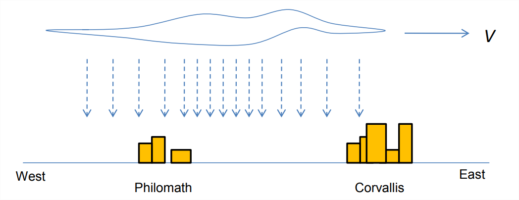
Figure \(\PageIndex{1}\): A rain storm moving eastward from Philomath to Corvallis.
- Proving more identities Prove the following:
- \((\vec{u} \times \vec{v}) \cdot(\vec{w} \times \vec{x})=(\vec{u} \cdot \vec{w})(\vec{v} \cdot \vec{x})-(\vec{u} \cdot \vec{x})(\vec{v} \cdot \vec{w})\)
- \(\vec{\nabla} \cdot(\vec{u} \times \vec{v})=\vec{v} \cdot(\vec{\nabla} \times \vec{u})-\vec{u} \cdot(\vec{\nabla} \times \vec{v})\)
- Streamlines and strains in a 2D flow A 2D steady flow has components \(\vec{u}= y\), \(\vec{v} = x\).
- Compute the streamfunction and show that the streamlines are hyperbolas: \(x^2 −y^2 = const\).
- Sketch a few representative streamlines, showing the direction of the flow.
- Compute the vorticity vector \(\vec{\omega}\) and the strain tensor \(\underset{\sim}{e}\).
- Compute the eigenvalues and eigenvectors of \(\underset{\sim}{e}\). Choose the eigenvectors to have unit length.
- Confirm that the eigenvectors are orthogonal.
- Form the rotation matrix that diagonalizes \(\underset{\sim}{e}\), ensuring that its determinant is \(\pm 1\) (reorder the eigenvalues and eigenvectors if necessary).
- Describe the rotation that this matrix represents. Give both angle and axis of rotation. (If this is not clear, try reordering the eigenvalues and eigenvectors.)
- Use your rotation matrix to diagonalize the strain tensor.
- Identify the principal axes and principal strains. Indicate these with arrows on your sketch from part 2.
- Characterize the principal strains as extensional or compressive.
- An isolated vortex An isolated vortex is one such that the circulation in the limit \(r\rightarrow\inf\) is zero. Consider an axisymmetric vortex (no dependence on the azimuthal angle \(\theta\)) for which the azimuthal velocity \(u_\theta\) is proportional to \(r^{-\alpha}\). What is the range of possible values of the exponent \(\alpha\) such that the circulation \(\Gamma(r)\) is finite as \(r\rightarrow\inf\)?
- The Rankine vortex A Rankine vortex has angular velocity \(\dot{\theta}\) for \(0\leq r \leq R\), and is irrotational for larger \(r\).
- Conservation of property \(X\) Suppose that \(X\) is the concentration of “something” per unit mass of fluid.
- Show that the concentration per unit volume is \(\rho X\), where \(\rho\) is the density of the fluid.
- Now suppose that the flux of \(X\) is given by \[\vec{F}_{X}=-\rho \gamma \vec{\nabla} X, \nonumber \] where \(\gamma\) is a scalar. Write down a Lagrangian conservation equation stating that the net amount of \(X\) in a fluid parcel changes according to the flux normal to its surface. (More specifically, the net \(X\) increases if the total flux through the surface is inward, and vice versa.)
- Assuming that mass is conserved, show that \(X\) must obey this equation: \[\frac{\partial X}{\partial t}+\vec{u} \cdot \vec{\nabla} X=\frac{1}{\rho} \vec{\nabla} \cdot(\rho \gamma \vec{\nabla} X). \nonumber \]
- Force on a small cube
- Compute the net contact force (per unit volume) on a cube with edge length \(\Delta\) in the limit \(\Delta\rightarrow 0\). Do this by integrating the stress vector \(\vec{f}=\hat{n}\underset{\sim}{\tau}\) over all 6 surfaces. Follow the sequence of steps we used in section 4.2.3 to compute the net volume flux out of a cube.
- Obtain the same result using the generalized divergence theorem.
- Preserving diagonality Under what conditions does a diagonal tensor remain diagonal after an arbitrary coordinate rotation \(\underset{\sim}{C}\)? [Hint: First assume that \(A_{11}\) = \(A_{22}\) = \(A_{33}\), and show that the tensor remains diagonal after an arbitrary rotation. Now, are there any other diagonal matrices that remain diagonal after an arbitrary rotation? Pick an easy rotation, one for which you can calculate \(\underset{\sim}{A}^\prime\) explicitly. Identify the conditions under which it is diagonal. (You may want to review your answer to exercise 10.5.) Now pick a different simple rotation and repeat the argument. If you can show that diagonality is preserved for these two particular rotations only if \(A_{11}\) = \(A_{22}\) = \(A_{33}\), then you have shown that diagonality is preserved for every rotation only if \(A_{11}\) = \(A_{22}\) = \(A_{33}\).]
- River flow In this problem you will use the Navier-Stokes equation, together with a list of simplifying assumptions, to predict the flow profile of the Willamette River as it flows past Corvallis (Figure \(\PageIndex{2}\)).
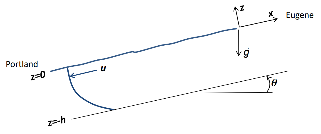
Figure \(\PageIndex{2}\): Definition sketch for the Willamette River, which flows northward between Eugene and Portland, Oregon. - Set up the equation for the flow velocity parallel to the bottom (\(u\)) as a function of perpendicular distance from the surface (\(z\)). Apply the appropriate boundary conditions and solve for \(u(z)\). [Hint: Two coordinate systems are useful here: gravity-aligned and tilted so that \(\hat{e}^{(x)}\) is parallel to the bottom. Although the gravity vector is simplest in gravity - aligned coordinates, everything else is simpler in tilted coordinates. So, solve the equations in the tilted coordinate system after performing the appropriate rotation to express \(\vec{g}\) in those coordinates.] Assume the following:
- The flow obeys the Navier - Stokes equation for an incompressible flow ( \(\vec{\nabla}\cdot\vec{u}=0\)).
- The current is steady (independent of time), so that \(\partial/\partial t\) of anything is zero.
- The density is uniform (\(\rho=\rho_0\)).
- The current is a parallel shear flow \(\vec{u}=u(z)\hat{e}^{(x)}\) in a coordinate frame parallel to the bottom.
- No fluid property varies in the direction parallel to the bottom (\(\partial/\partial x =0\)).
- No fluid property varies in the cross - stream (\(y\)) direction.
- At the river bottom, \(u = 0\).
- At the surface, \(du/dz = 0\). (This is true when wind effects are not important.)
- What is the velocity at the surface? Give a numerical value based on the following parameter values:
- The mean grade (slope) of the Willamette River is 43 cm per km.
- The kinematic viscosity \(ν\) = \(\mu/\rho\) = 10−6 m2/s.
- The water depth \(h\) = 2 m.
- The vertical gravitational acceleration \(g\) = 9.8 m/s2.
- Does your result seem consistent with the observed velocity?
- Suppose that frictional effects are supplied not by molecular viscosity but by a much larger “effective” viscosity due to turbulence (see section 6.3.5). If this turbulent viscosity is 10−2m2s−1, what is the maximum flow speed? Verify that this velocity is more consistent with observations than the value you obtained in 29.2.
- Set up the equation for the flow velocity parallel to the bottom (\(u\)) as a function of perpendicular distance from the surface (\(z\)). Apply the appropriate boundary conditions and solve for \(u(z)\). [Hint: Two coordinate systems are useful here: gravity-aligned and tilted so that \(\hat{e}^{(x)}\) is parallel to the bottom. Although the gravity vector is simplest in gravity - aligned coordinates, everything else is simpler in tilted coordinates. So, solve the equations in the tilted coordinate system after performing the appropriate rotation to express \(\vec{g}\) in those coordinates.] Assume the following:
- Pressure drop and surface deflection in a Rankine vortex Consider the Rankine vortex, a steady, axisymmetric vortex whose velocity is purely azimuthal and is given by \[u_{\theta}(r)=\left\{\begin{array}{cl}
\dot{\theta} r & \text { for } r \leq R \\
\dot{\theta} R^{2} r^{-1} & \text {for } r \geq R
\end{array}\right. \nonumber \] (see exercise 25).- Beginning with the radial velocity equation for inviscid, homogeneous flow (Appendix I.1), \[\frac{D u_{r}}{D t}=\frac{u_{\theta}^{2}}{r}-\frac{1}{\rho_{0}} \frac{\partial p}{\partial r}, \nonumber \] write down a differential equation whose solution is the r-dependence of the pressure p(r) in a Rankine vortex.
- Solve the equation, requiring that \(p(r)\) be a continuous function. Sketch a graph of your solution. (We did the inner part, \(r < R\), in class. Your solution should include all \(r\).)
- Show that the pressure drop between \(r\) = \(\inf\) and \(r \)= 0 is \(\rho_0V^2\), where \(\rho_0\) is the density and \(V\) is the maximum value of the azimuthal velocity \(u_\theta\).
- Suppose that the Rankine vortex in 30.1 exists in a body of water with surface \(z = \eta(r)\), and that the vertical pressure gradient is hydrostatic. Compute the profile of surface elevation \(\eta(r)\). You can assume that, as \(r\rightarrow\inf\), both the surface pressure and the surface displacement approach zero. Show that \(\eta(0) = −V^2/g\), and sketch \(\eta(r)\).
- Consider the angular frequency \(\dot{\theta}\). How does the surface deflection \(\eta(0)\) vary with this frequency, all else being equal?
- Kitchen sink experiment Obtain a clear cylindrical container such as a big measuring cup. A glass coffee mug will do, but the bigger the better. You’ll also need a watch (or other way to measure seconds), a ruler, and something to stir with. Fill the container about 3/4 full with water. Stir the water until it is rotating evenly, and notice that the water surface is depressed at the center and elevated at the outside. Notice also that the faster you stir, the greater the depression/elevation. Your objective is to determine how the depression (or elevation) depends on the frequency of stirring. It will be a power - law dependence, i.e., depression/elevation will be proportional to frequency, or frequency2, or frequency3 or something, and you’re going to determine the exponent. Submit a clear description of your method, results and interpretation.
- Devise some way to measure the depression/elevation to within, say, 1 mm. This could be the depression, the elevation, or the difference between the two, whichever you find easiest to measure. Call this distance \(h\). [Here is one way: with the fluid motionless, mark the level on the outside of the container. Then, with the fluid turning, mark the elevation again and measure the difference.]
- Devise a way to measure the frequency of stirring (e.g., 1 stir per second). You can probably use your watch or some app on your phone. Call that frequency \(f\).
- Make the measurement at several frequencies and plot a graph of logh versus log \(f\). Try at least 4 frequencies (more is better) covering a wide range (a factor of 4 or more, say).
- If \(h = a f^n\), where \(a\) and \(n\) are constants, then this graph should give a straight line. Fit a straight line through your measurements, determine its slope and intercept, and from that information estimate values for \(a\) and \(n\). (Do not forget to include units!)
- Compare your estimate of n with the theoretical prediction developed in exercise 30 for the Rankine vortex. List possible reasons why this comparison may be imperfect. (This should include both measurement inaccuracies and physical assumptions that may be wrong.) Say which you think is most likely to be important.
- The Froude number The Froude2 number is important in hydraulic channel flows. It is defined as \[F=\frac{|u|}{\sqrt{g H}}, \nonumber \] where \(u(x)\) is the flow velocity in a unidirectional current (a river, say), \(g\) is gravity and \(H(x)\) is the depth of the fluid. Consider a channel of uniform width where the flow velocity varies inversely with depth so as to conserve the volume flux: \(uH = const\).3 Compute the Froude number for each of the following situations. Approximate \(g\) as 10 ms-2 for simplicity.
- \(u=1 m s^{-1}, H=0.1 m\)
- Depth \(H\) increases to 0.4 m (with the same volume flux).
- Depth \(H\) decreases to 0.025 m.
- Effects of surface tension on surface waves
- Derive the dispersion relation \(\omega = \omega (k)\) for surface waves in the presence of surface tension. Surface tension imposes an effective pressure at the surface given by \(p = −\sigma \nabla^2\eta\), where \(\sigma\) is a constant. This alters the surface boundary condition on pressure. Aside from this, make the same assumptions we made in class: the fluid is homogeneous and inviscid, and there is no variation in the \(y\) - direction.
- Show that the frequency \(\omega\) is increased by a factor \(\sqrt{1+\sigma k^2/\rho_0g}\) over the case without surface tension.
- Compute the wavelength of waves for which the second term in the dispersion relation equals the first (i.e., the contribution from surface tension equals that from gravity). Give a numerical value for this wavelength for the water/air interface (\(\sigma/\rho_0 = 7.4\times 10^{−5}m^3s^{−2}\)). Waves shorter than this are called capillary waves.
- Mass conservation in a channel flow
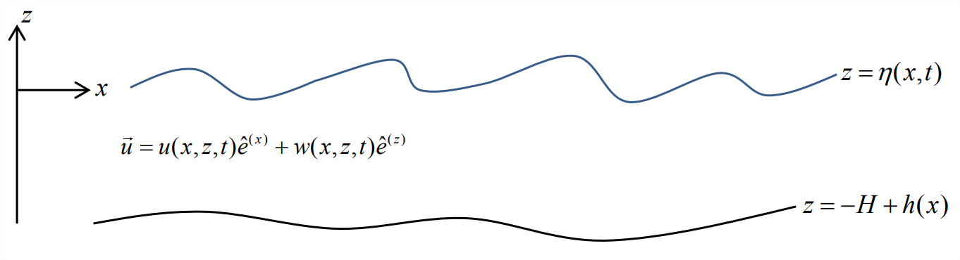
Figure \(\PageIndex{3}\): Definition sketch for two-dimensional channel flow. - Consider inviscid, incompressible, 2 - dimensional flow (independent of \(y\)) in a channel with a corrugated, impermeable bottom \(z = −H +h(x)\) and an undulating surface \(z = \eta(x,t)\) (Figure \(\PageIndex{3}\)). Integrate the divergence vertically over the water column: \[\int_{-H+h(x)}^{\eta(x, t)}\left(\frac{\partial u}{\partial x}+\frac{\partial w}{\partial z}\right) d z, \nonumber \] simplify where possible and set the result equal to zero. Use the result to show that \[\frac{\partial \eta}{\partial t}=-\frac{\partial}{\partial x} \int_{-H+h(x)}^{\eta(x, t)} u d z. \nonumber \] [Hints: For the first term, use the 1 - dimensional form of Leibniz’ rule Equation 6.1.3 to bring the partial derivative outside the integral. Simplify the second term by using the appropriate boundary conditions. Do not assume that the disturbance is small-amplitude.]
- What difference does it make to 34.1 if the fluid is viscous, i.e., if the current goes to zero at the bottom boundary?
1Corvallis, Oregon is the home of Oregon State University, and Philomath is a town a few miles to the west. A few miles further to the west is the Pacific ocean, which makes for a lot of rainstorms.
2Rhymes with “food”.
3Hence the saying “Still waters run deep.”