6.4: The Durand and Condolios (1952) School

6.4.1 Soleil & Ballade (1952)

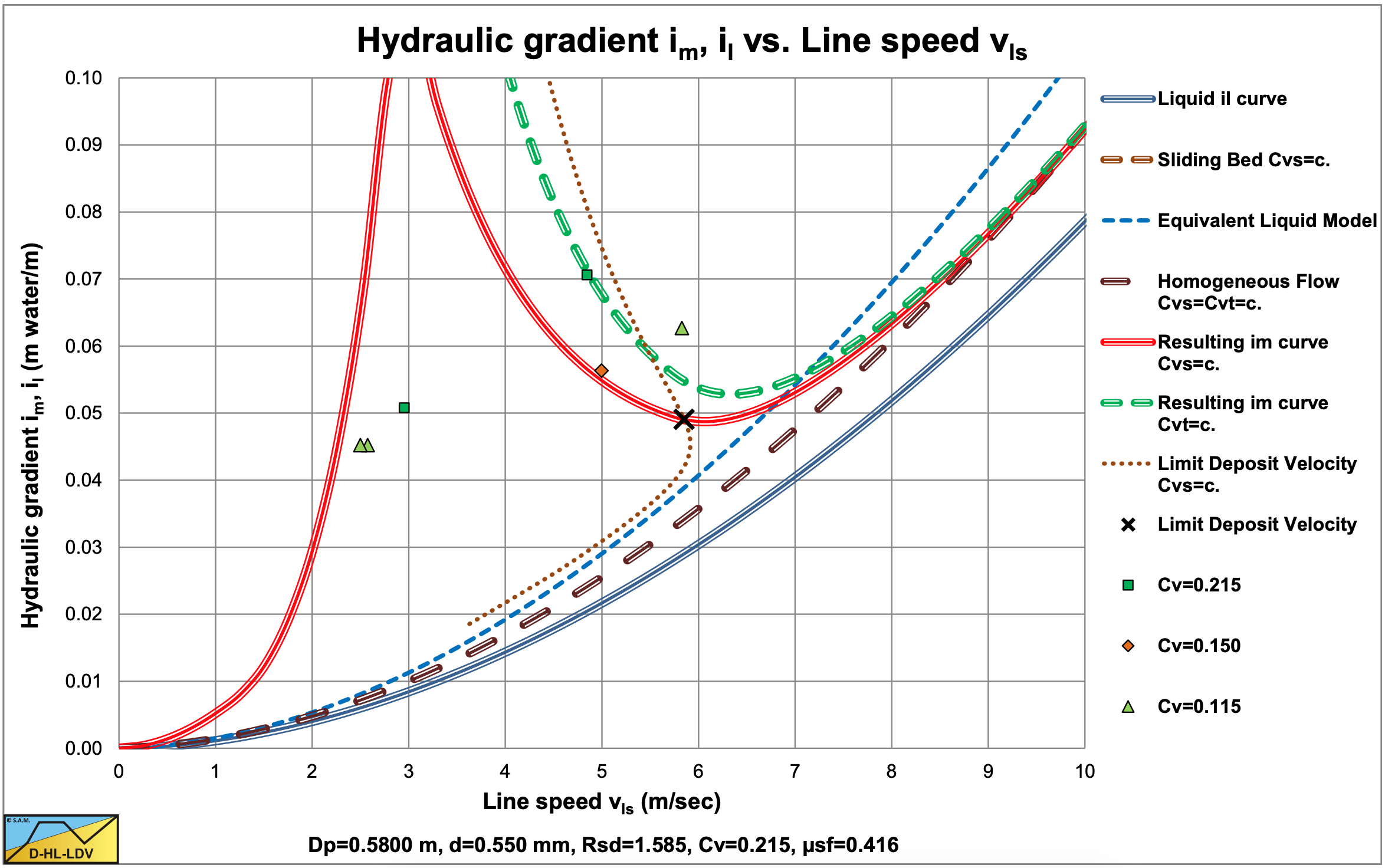
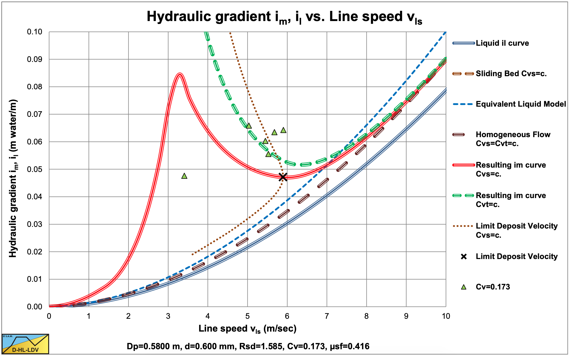
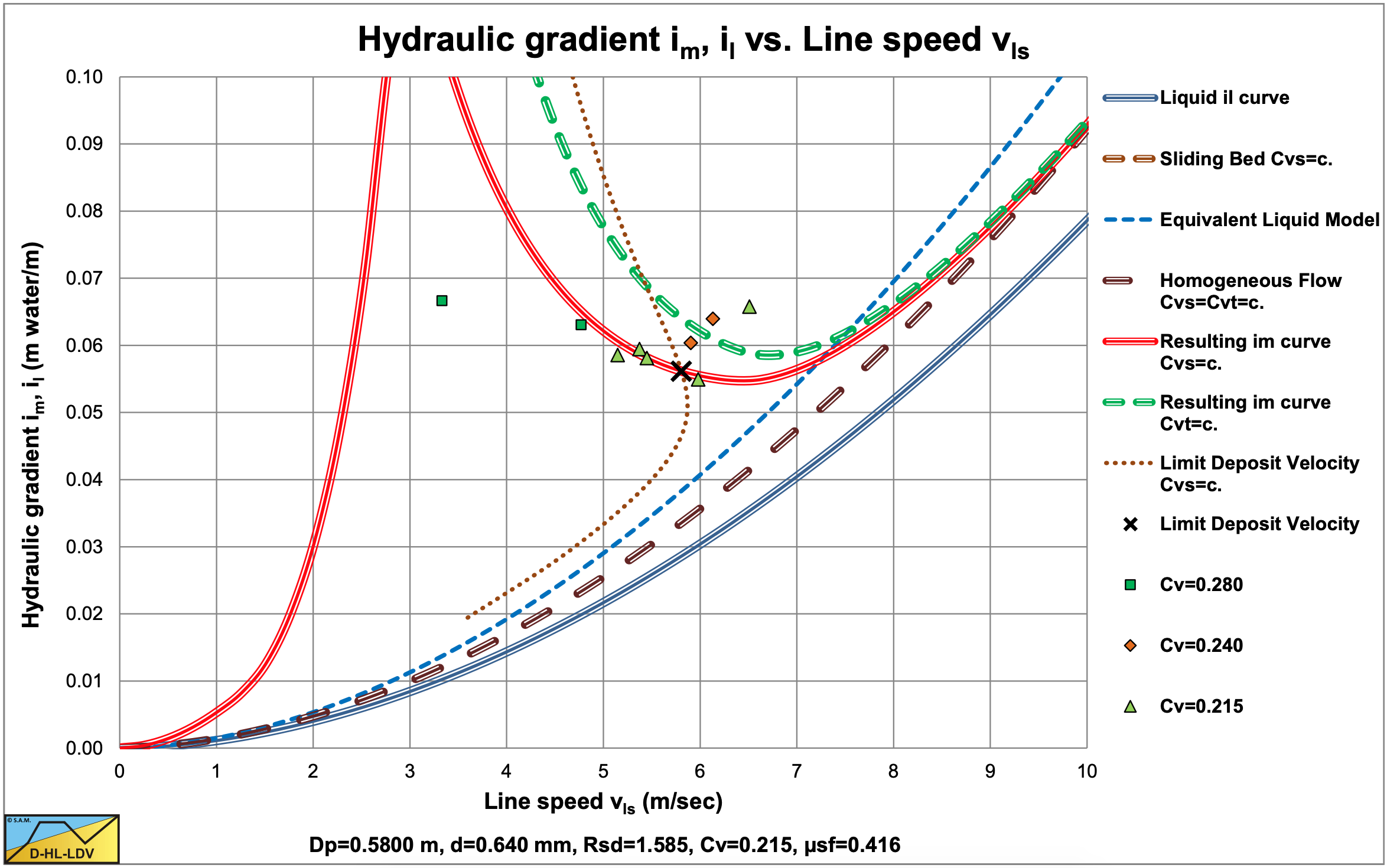
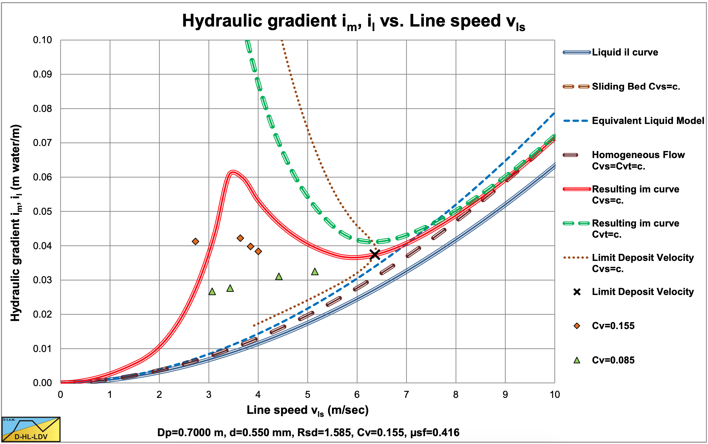
Soleil & Ballade (1952) carried out experiments on a real dredge with pipe diameters of D_p=0.58 m and D_p=0.70 m. The sands used had diameters of d=0.55 mm, d=0.60 mm and d=0.64 mm. The flows for both pipe diameters were in the same range, resulting in lower line speeds for the larger pipe diameter.

Most probably, the concentrations measured were spatial volumetric concentrations. Most experiments were just above the Limit Deposit Velocity or just below. The experiments below the LDV were in a transition between a stationary bed and the heterogeneous regime. Although there is a lot of scatter, the experiments are shown here, because the number of experimental data with large diameter pipes is very limited. Durand & Condolios (1952) used these experiments in their analysis.

Most experiments in the D_p=0.70 m pipe were carried out in this transition zone, while most experiments in the D_p=0.58 m pipe were carried out in the heterogeneous regime. Again the experiments point to spatial concentration measurements, since the delivered concentrations of the same values at the low line speeds would have given a sliding bed.

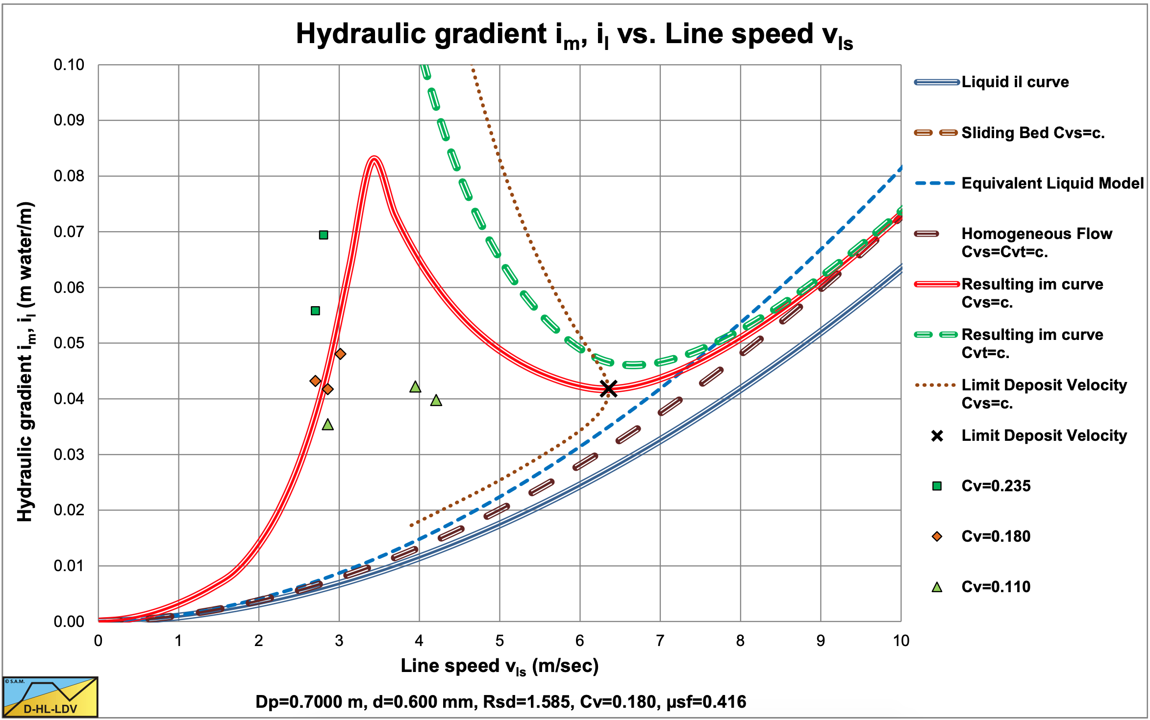
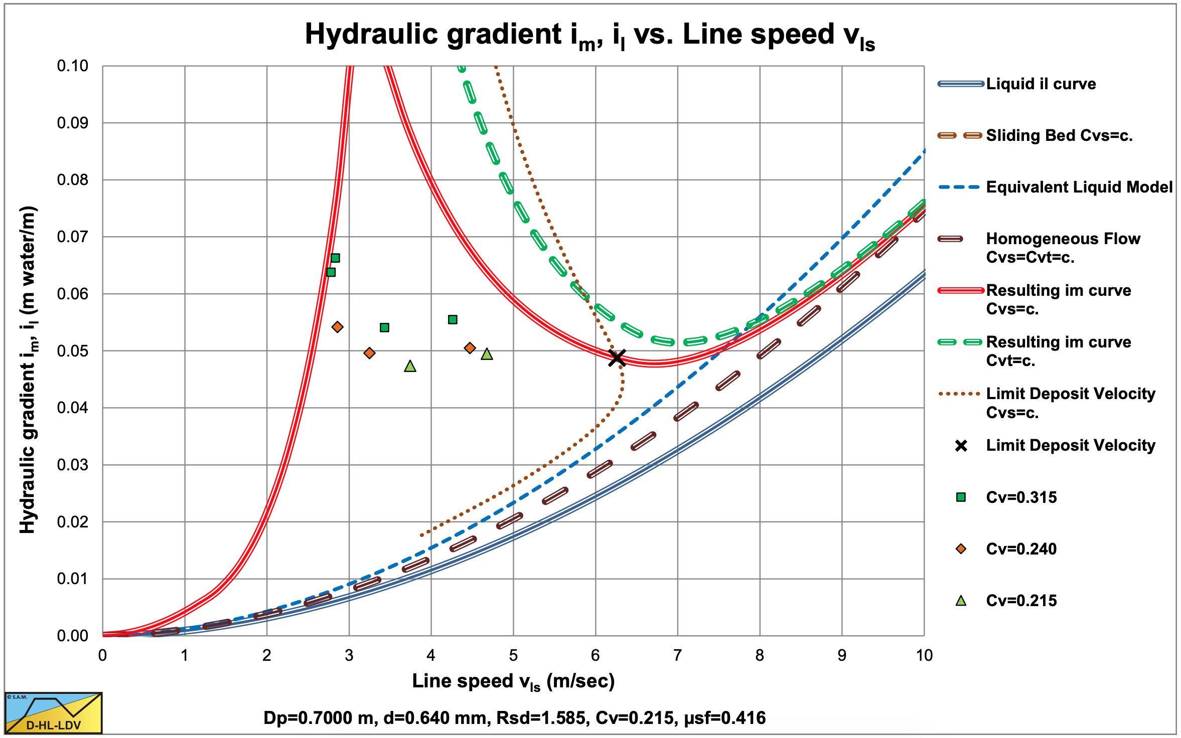
Figure 6.4-1, Figure 6.4-2 and Figure 6.4-3 show the experiments in the D_p=0.58 m pipe. Most data points are in the heterogeneous flow regime, but some at low line speeds are in the transition between a fixed bed and the heterogeneous flow regime around the LDV. Both the data points and the DHLLDV Framework prediction do not show a sliding bed.

Figure 6.4-4, Figure 6.4-5 and Figure 6.4-6 show the experiments in the D_p=0.70 m pipe. Most data points are in the transition between a fixed bed and the heterogeneous flow regime below the LDV. Both the data points and the DHLLDV Framework prediction do not show a sliding bed.

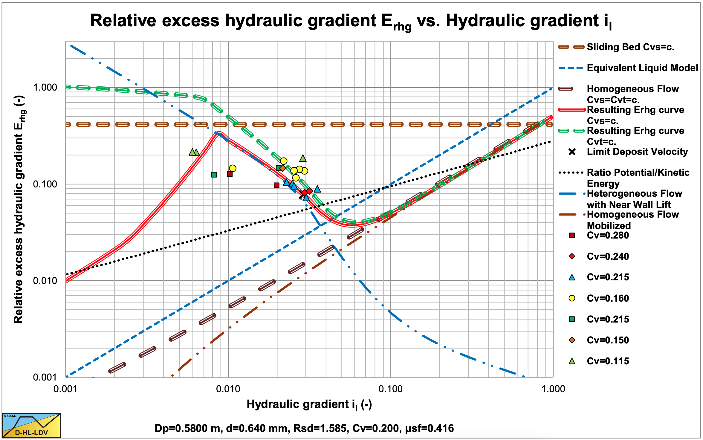
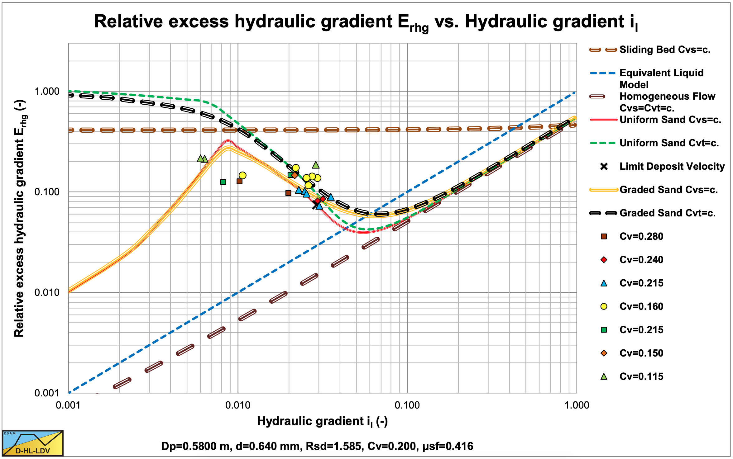
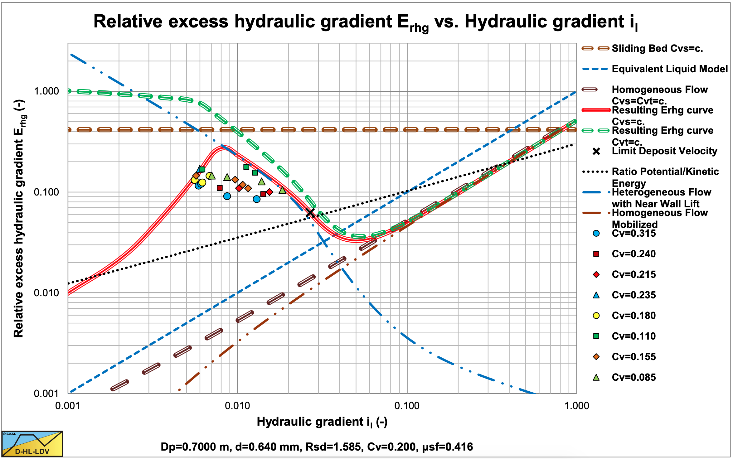
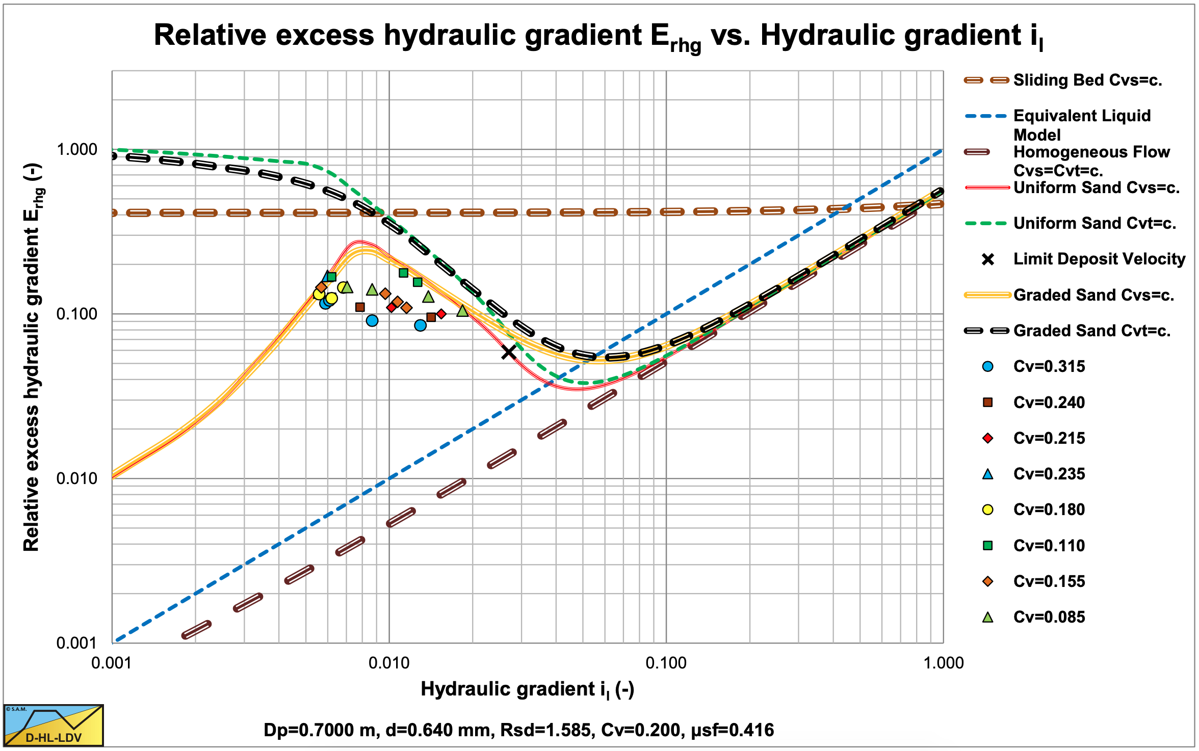
Figure 6.4-7 and Figure 6.4-8 show the relative excess hydraulic gradient E_rhg in the D_p=0.58 m pipe of all experiments (all particle sizes) for a uniform and a graded prediction of the DHLLDV Framework. For the line speed range considered there is hardly a difference between the uniform and the graded prediction.

Figure 6.4-9 and Figure 6.4-10 show the relative excess hydraulic gradient E_rhg in the D_p=0.70 m pipe of all experiments (all particle sizes) for a uniform and a graded prediction of the DHLLDV Framework. For the line speed range considered there is hardly a difference between the uniform and the graded prediction.

In general the experiments match the DHLLDV Framework, however, the transition between the stationary bed regime and the heterogeneous regime seems to be more smooth and does not show the peak. This makes sense, since the DHLLDV Framework does not consider suspension only sheet flow at the top of the bed, while in reality above the bed and above the sheet flow layer there will be suspension.

For practical purposes the line speeds are rather low. In real life line speeds above the LDV would be applied.

Figure 6.4-1: Experiments with sand d=0.55 mm and a pipe diameter of D_p=0.58 m.

Figure 6.4-2: Experiments with sand d=0.60 mm and a pipe diameter of D_p=0.58 m.

Figure 6.4-3: Experiments with sand d=0.64 mm and a pipe diameter of D_p=0.58 m.

Figure 6.4-4: Experiments with sand d=0.55 mm and a pipe diameter of D_p=0.70 m.

Figure 6.4-5: Experiments with sand d=0.60 mm and a pipe diameter of D_p=0.70 m.

Figure 6.4-6: Experiments with sand d=0.64 mm and a pipe diameter of D_p=0.70 m.

Figure 6.4-7: Experiments with sands in a pipe diameter of D_p=0.58 m, uniform.

Figure 6.4-8: Experiments with sands in a pipe diameter of D_p=0.58 m, graded.

Figure 6.4-9: Experiments with sands in a pipe diameter of D_p=0.70 m, uniform.

Figure 6.4-10: Experiments with sands in a pipe diameter of D_p=0.70 m, graded.

6.4.2 Durand & Condolios (1952), (1956), Durand (1953) and Gibert (1960)

Durand & Condolios (1952) and Durand (1953) carried out experiments in solids (mostly sand and gravel) with a d₅₀ between 0.18 mm and 22.5 mm in pipes with a diameter D_p from 40 to 700 mm and volumetric concentrations C_vt from 2% to 22%. The large pipe diameter experiments (D_p=0.58 m and D_p=0.70 m) were carried out by Soleil & Ballade (1952) on a real dredge. Gibert (1960) analyzed the data of Durand & Condolios (1952) and summarized the results. A possible parameter to define the solids effect is the relative excess pressure loss p_er:

\[\ \mathrm{p}_{\mathrm{er}}=\left(\frac{\mathrm{i}_{\mathrm{m}}-\mathrm{i}_{\mathrm{l}}}{\mathrm{i}_{\mathrm{l}}}\right)\]

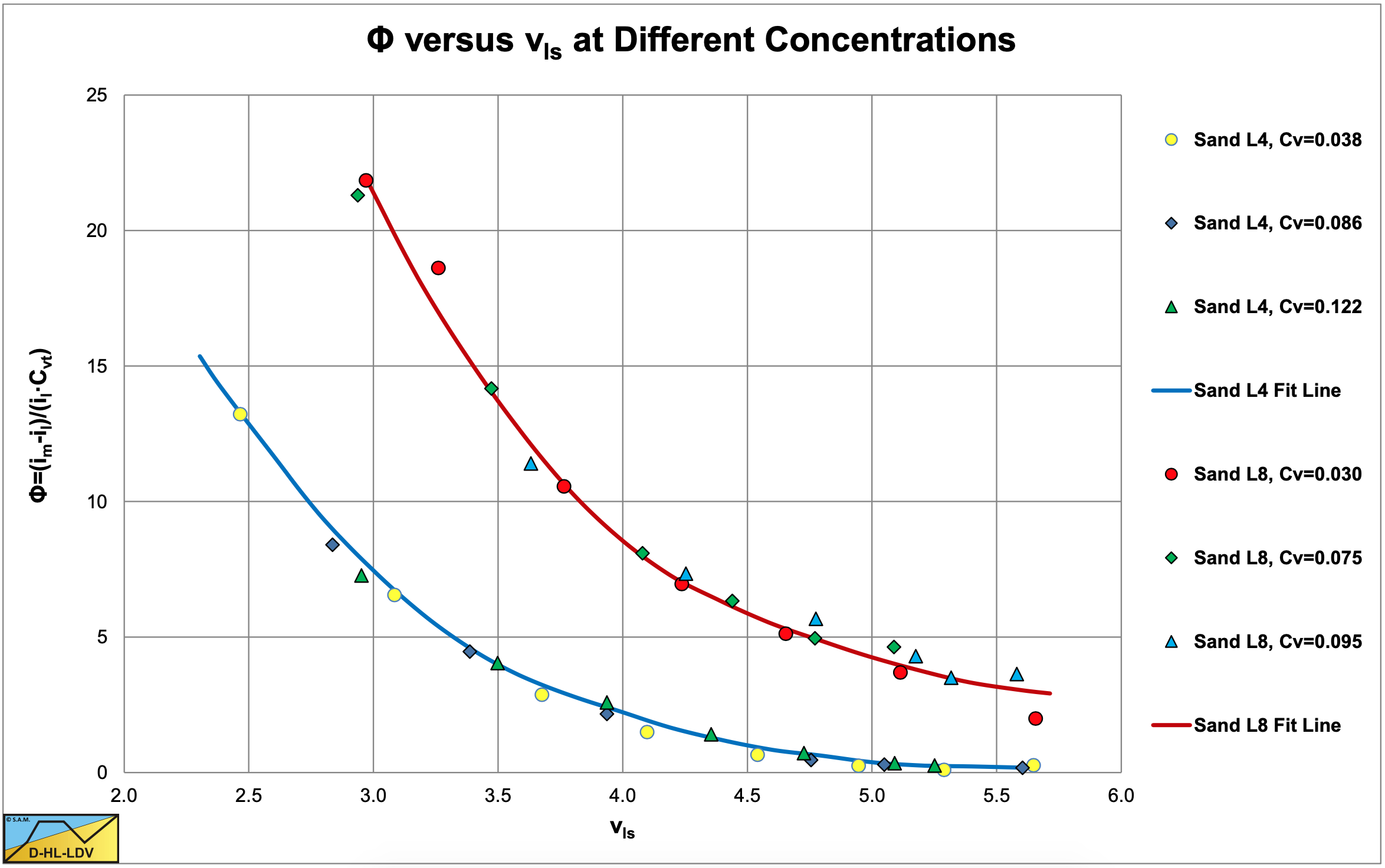
The first step Durand & Condolios (1952) carried out was to define a parameter Φ, which is the relative excess pressure loss p_er divided by the concentration C_vt and plot the pressure loss data of two sands with the parameter Φ versus the line speed v_ls. The transport regime of the data points is heterogeneous, which means that there will not be much difference between the spatial and the transport concentration. The parameter Φ was defined as:

\[\ \Phi=\left(\frac{\mathrm{p}_{\mathrm{er}}}{\mathrm{C}_{\mathrm{v}}}\right)=\left(\frac{\mathrm{i}_{\mathrm{m}}-\mathrm{i}_{\mathrm{l}}}{\mathrm{i}_{\mathrm{l}} \cdot \mathrm{C}_{\mathrm{v} \mathrm{t}}}\right)\]

With, in general for the hydraulic gradient i:

\[\ \mathrm{i}=\frac{\Delta \mathrm{p}}{\rho_{\mathrm{l}} \cdot \mathrm{g} \cdot \Delta \mathrm{L}}\]

The volumetric concentration C_vt is the transport concentration, which for high line speeds and heterogeneous transport is considered to be almost equal to the spatial volumetric concentration C_vs, assuming that the slip between the particles and the carrying liquid can be neglected. Figure 6.4-11 shows the resulting curves of experiments at different volumetric concentrations in the heterogeneous regime, where the data points of different concentrations apparently converge to one curve. The data points of the two types of sand still result in two different curves. Whether the linear relationship between the relative solids excess pressure is exactly linear with the concentration C_vt requires more experiments and especially experiments at much higher concentrations in order to see if hindered settling will have an effect, but for low concentrations the conclusion of Durand & Condolios (1952) seems valid.

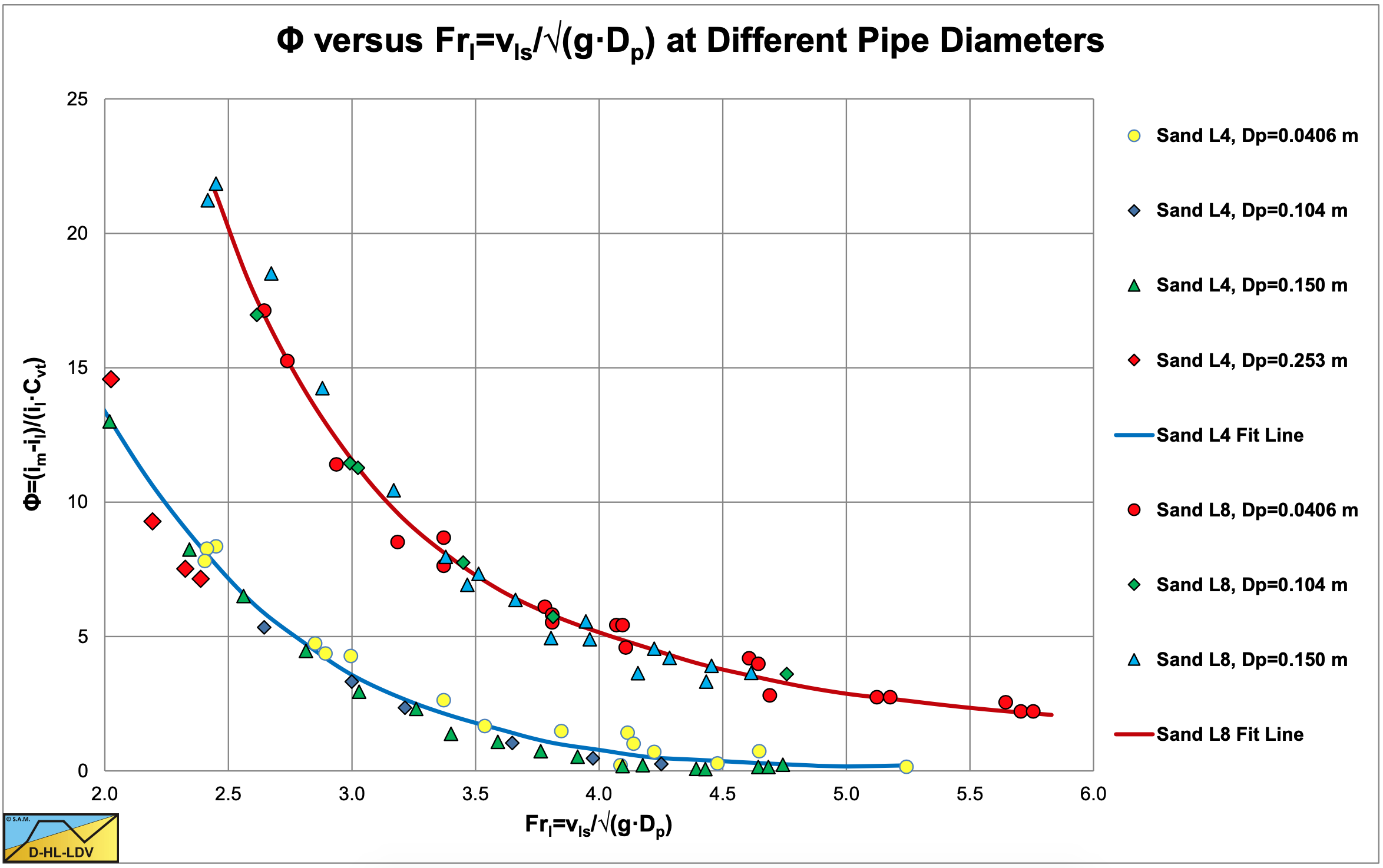
The second step Durand & Condolios carried out was to investigate the influence of the pipe diameter D_p. Instead of using the line speed v_ls on the horizontal axis, they suggested to use the Froude number of the flow; \(\ \mathrm{F r}_{\mathrm{f} \mathrm{l}}=\mathrm{v}_{\mathrm{l} \mathrm{s}} / \sqrt{\mathrm{g} \cdot \mathrm{D}_{\mathrm{p}}}\). Figure 6.4-12 shows how the data points of two sands and 4 pipe diameters converge to two curves, one for each sand. Within the range of the pipe diameters applied and the range of the particle diameters applied, the assumption of Durand & Condolios (1952) that the parameter Φ is proportional to the square root of the pipe diameter and reversely proportional to the flow Froude number, seems very reasonable. Whether this proportionality is linear or to a certain power close to unity is subject to further investigation.

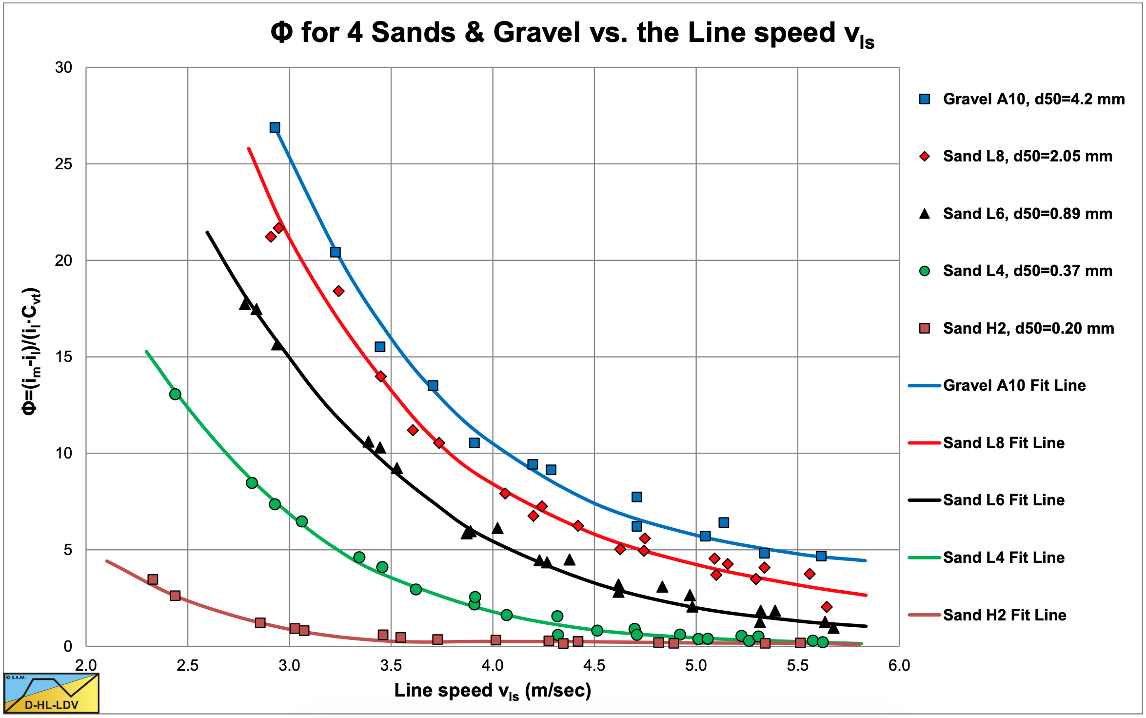
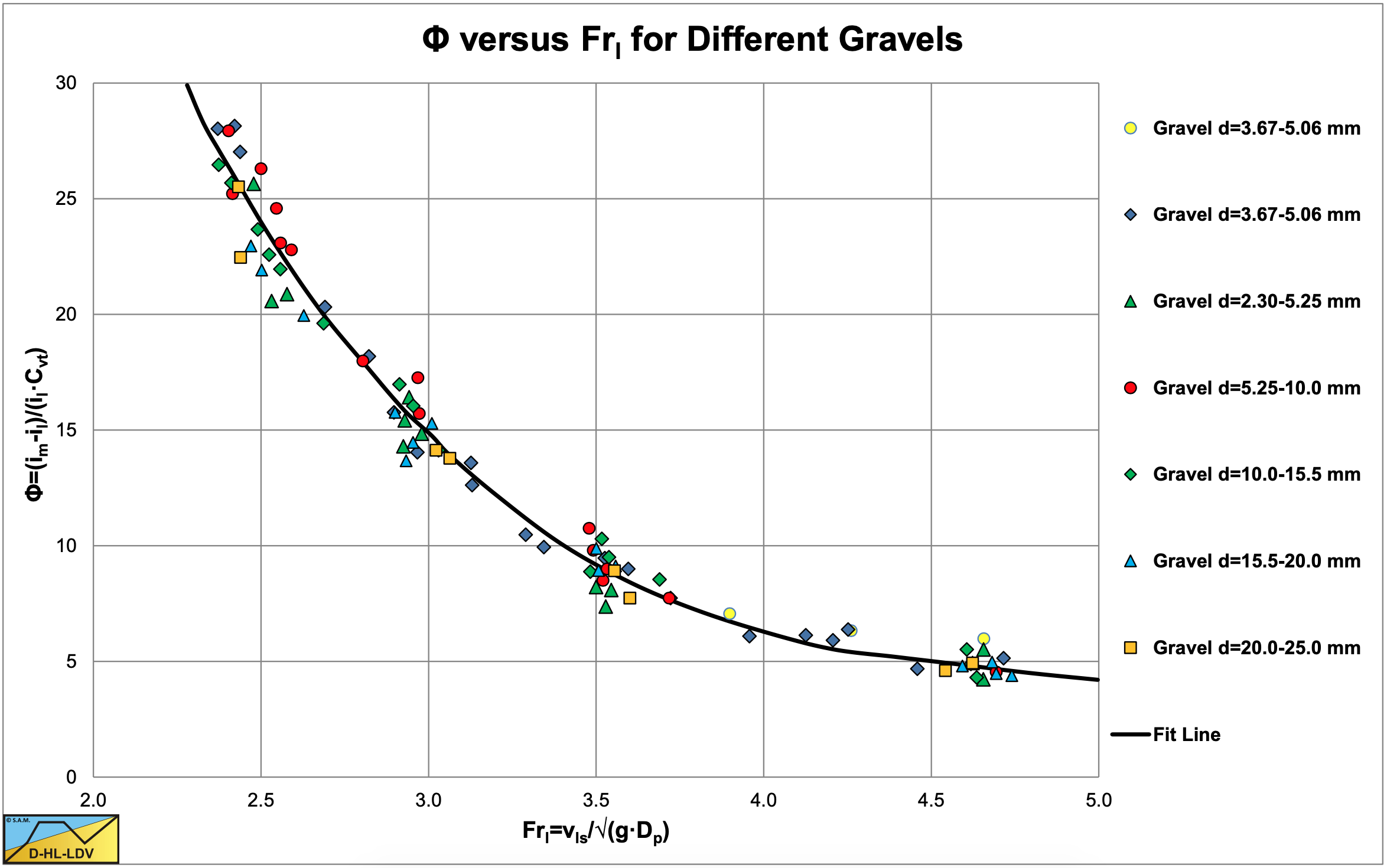
Now that proportionalities have been found between the parameter Φ on one hand and the concentration C_vt and the pipe diameter D_p on the other hand, Durand & Condolios (1952) investigated the influence of the particle diameter. Figure 6.4-13 shows the results of experiments in 4 sands and one gravel ranging from a d₅₀=0.20 mm to a d₅₀=4.2 mm in a D_p=0.150 m pipe. Figure 6.4-14 shows the results of 7 gravels.

Figure 6.4-14 shows that in the case of gravels the relation between Φ and Fr_fl does not depend on the particle size, but Figure 6.4-13 shows that for smaller particles it does. A parameter that shows such a behavior is the drag coefficient C_D as used to determine the terminal settling velocity v_t of the particles. For small particles the drag coefficient depends strongly on the particle diameter, but for particles larger than about 1 mm, the drag coefficient is a constant with a value of about 0.445 for spheres and up to about 1-1.5 for angular sand grains. Instead of using the drag coefficient directly, Durand & Condolios (1952) choose to use the particle Froude number \(\ \mathrm{F r}_{\mathrm{p}}=\mathrm{v}_{\mathrm{t}} / \sqrt{\mathrm{g} \cdot \mathrm{d}}\). It cannot be emphasized enough that this particle Froude number is different from the reciprocal of the drag coefficient C_D, although it is mixed up in many text books, together with some other errors, resulting in the wrong use and interpretation of the Durand & Condolios (1952) results.

Figure 6.4-11: Φ at different concentrations as a function of the line speed in a D_p=0.150 m pipe.

Figure 6.4-12: Φ at different pipe diameters as a function of the flow Froude number Fr_fl.

Figure 6.4-13: Φ as a function of v_ls for 4 sands and 1 gravel.

Figure 6.4-14: Φ as a function of Fr_fl in 7 gravels.

Figure 6.4-15: The relationship of the Durand & Condolios (1952) model, linear.

Figure 6.4-16: The relationship of the Durand & Condolios (1952) model, logarithmic.

Figure 6.4-17: The relationship of the Durand & Condolios (1952) and Gibert (1960) model, logarithmic. Here distinguished between experiments with a bed, sieved sand, mixed sand and natural sand.

Figure 6.4-18: The relationship of the Durand & Condolios (1952) and Gibert (1960) model, logarithmic. Here experiments with a bed.

In order to make the 5 curves in Figure 6.4-13 converge into one curve, Durand & Condolios (1952) extended the parameter on the horizontal axis with the particle Froude number to:

\[\ \Psi=\left(\frac{\mathrm{v}_{\mathrm{l s}}}{\sqrt{\mathrm{g} \cdot \mathrm{D}_{\mathrm{p}}}}\right)^{2} \cdot\left(\frac{\mathrm{v}_{\mathrm{t}}}{\sqrt{\mathrm{g} \cdot \mathrm{d}_{50}}}\right)^{-1}\]

With:

\[\ \mathrm{Fr}_{\mathrm{fl}}=\left(\frac{\mathrm{v}_{\mathrm{ls}}}{\sqrt{\mathrm{g} \cdot \mathrm{D}_{\mathrm{p}}}}\right)\quad\text{ and }\quad \mathrm{Fr}_{\mathrm{p}}=\frac{1}{\sqrt{\mathrm{C}_{\mathrm{x}}}}=\left(\frac{\mathrm{v}_{\mathrm{t}}}{\sqrt{\mathrm{g} \cdot \mathrm{d}_{50}}}\right)\quad\text{ and }\quad\mathrm{C}_{\mathrm{x}}=\frac{\mathrm{g} \cdot \mathrm{d}_{50}}{\mathrm{v}_{\mathrm{t}}^{2}}=\mathrm{Fr}_{\mathrm{p}}^{-2}\]

Which are the Froude number of the flow Fr_fl and the Froude number of the particle Fr_p, which also looks like a sort of reciprocal drag coefficient (but it’s not) , which will be explained later. The variable ψ can now also be written in terms of the two Froude numbers as defined above.

\[\ \Psi=\mathrm{F} \mathrm{r}_{\mathrm{fl}}^{\mathrm{2}} \cdot \mathrm{F} \mathrm{r}_{\mathrm{p}}^{-\mathrm{1}}\]

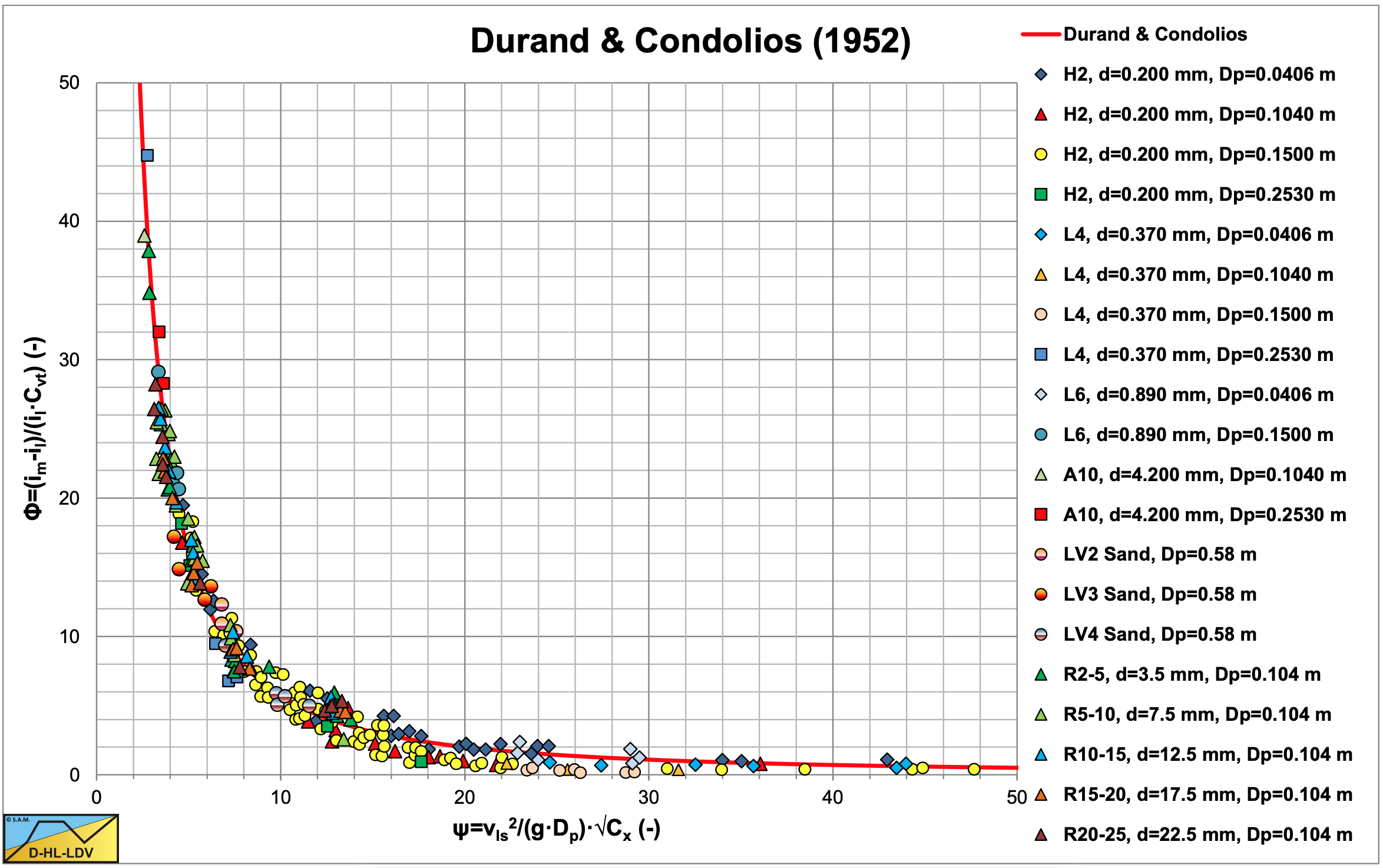
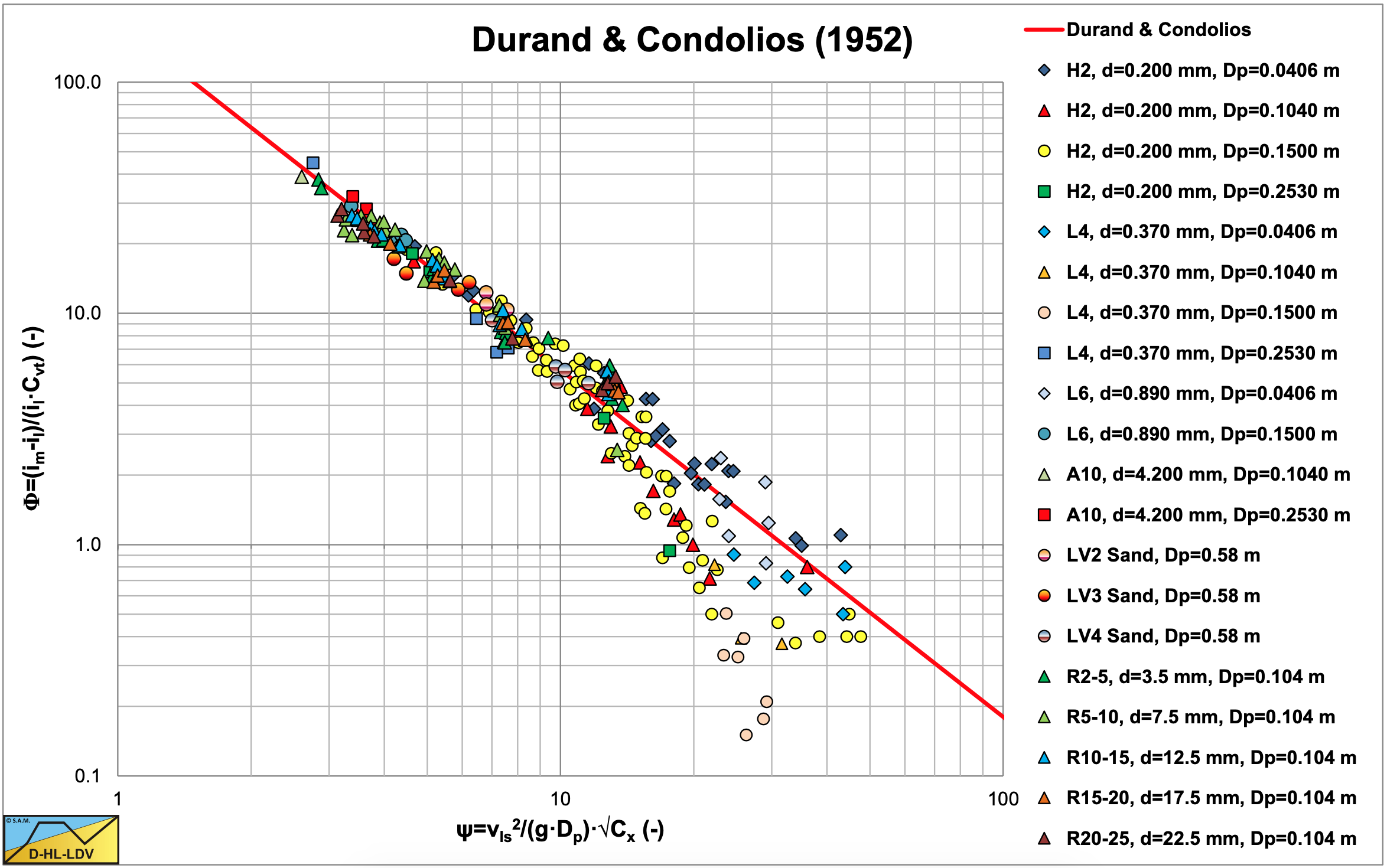
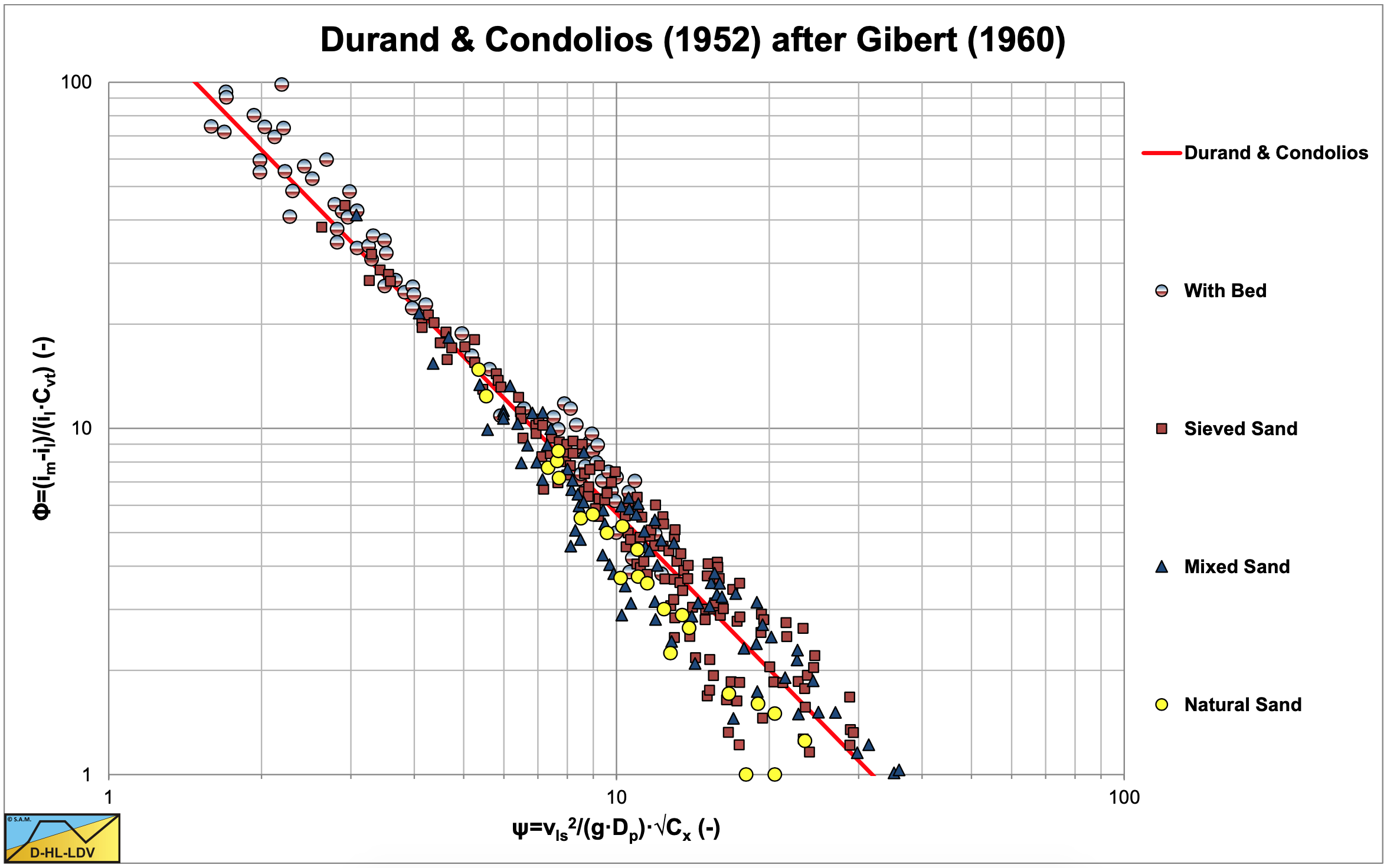
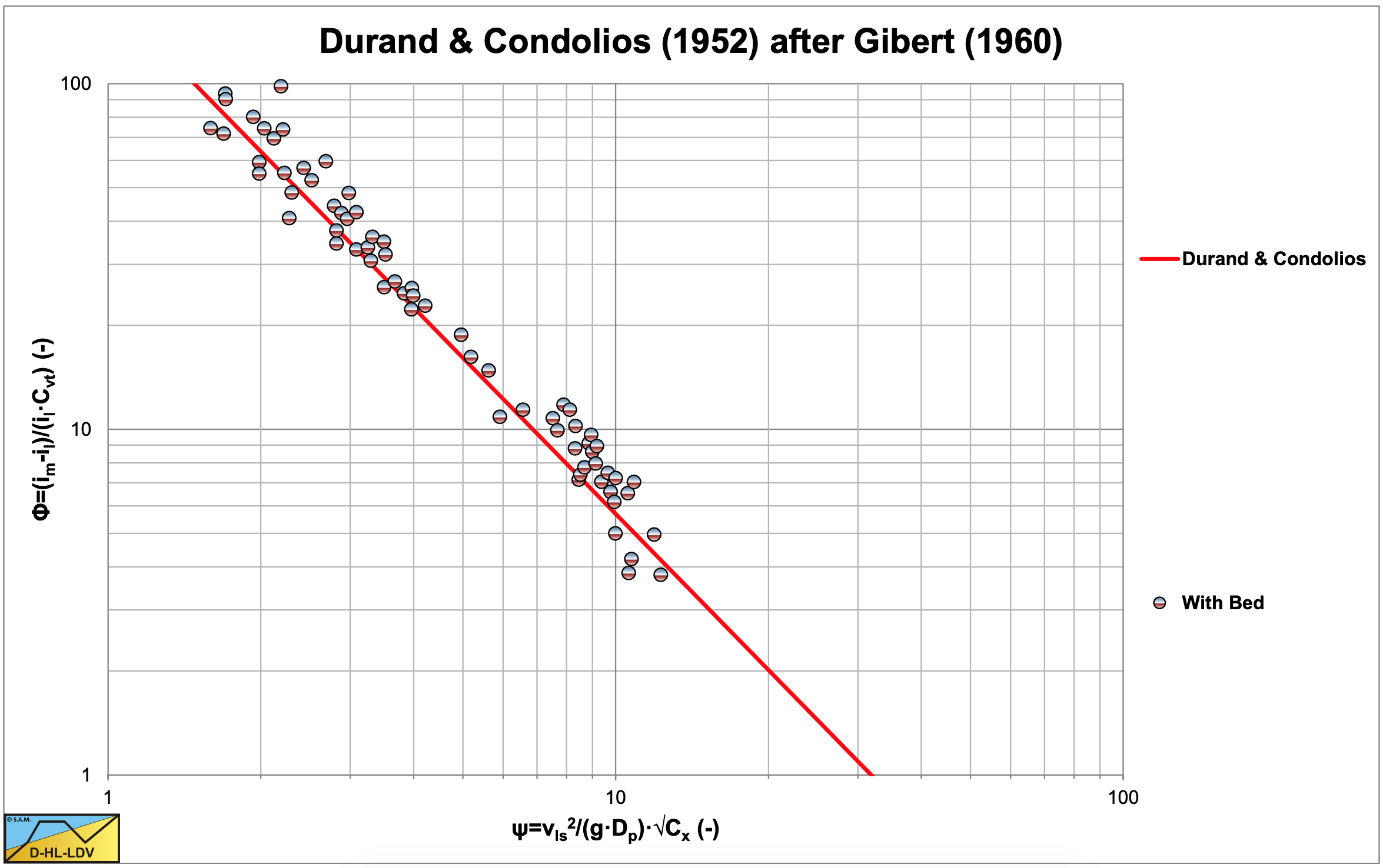
Durand & Condolios (1952) plotted all their data against this new parameter ψ as is shown in Figure 6.4-16 on linear scales and Figure 6.4-15 on logarithmic scales. The assumption of using the particle Froude number Frp seemed to be successful. Figure 6.4-17 shows the data points distinguished into 4 groups, experiments where a bed occurred, experiments with sieved sand, experiments with mixed sands and experiments with natural sands. It is obvious from this figure that also the data points from experiments with a bed occurring, follow the same fit curve, see Figure 6.4-18. The curves for different sands, pipe diameters and concentrations converged into one curve with the equation:

\[\ \Phi=\mathrm{K} \cdot \Psi^{-3 / 2}
\quad \text{ With : } \quad \mathrm{K}=\mathrm{1 7 6}\]

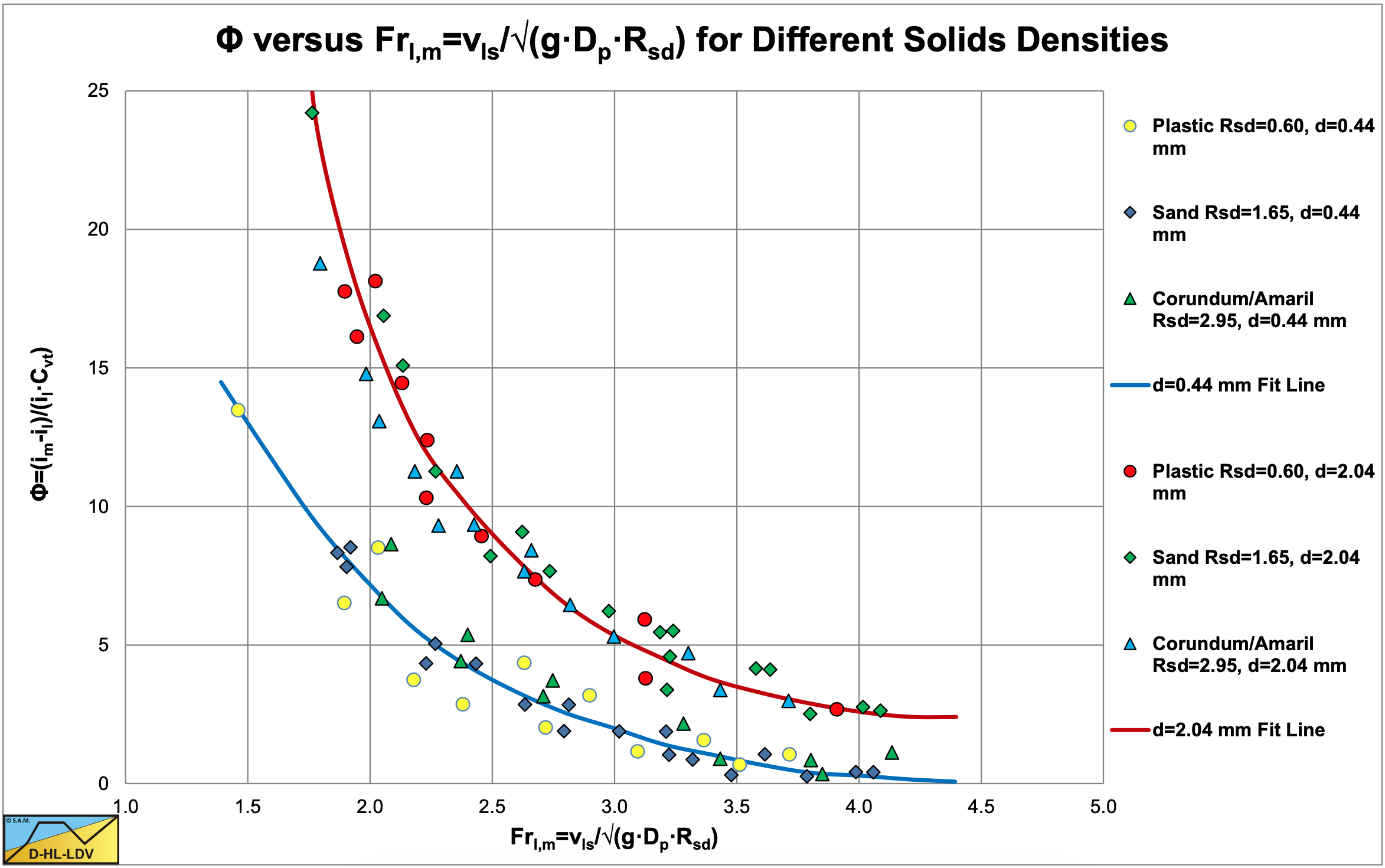
The constant of 176 is found from the original graph of Durand & Condolios (1952) (source Bain & Bonnington (1970)). The next step was to investigate the influence of the relative submerged density of the particles. Gibert (1960) reported on a set of experiments on plastic, sand and Corundum with 3 different relative densities. Figure 6.4-19 shows the results of these experiments.

By extending the flow Froude number Fr_fl, with the relative submerged density R_sd the data points converge to one curve for each particle diameter. The liquid flow Froude number Fr_fl is modified according to:

\[\ \mathrm{F r}_{\mathrm{fl}}=\frac{\mathrm{v}_{\mathrm{l s}}}{\sqrt{\mathrm{g} \cdot \mathrm{D}_{\mathrm{p}} \cdot \mathrm{R}_{\mathrm{s d}}}}\]

Applying this modified Froude number, nothing changes in the equation for sand with a relative submerged density of about R_sd=1.65, using in a new constant of 83 instead of 176 for K. The equation for the particle Froude number does not change according to Gibert (1960) because of the relative submerged density R_sd and remains:

\(\ \mathrm{F r}_{\mathrm{p}}=\mathrm{v}_{\mathrm{t}} / \sqrt{\mathrm{g} \cdot \mathrm{d}}\)

The final equation of Durand & Condolios (1952) and later Gibert (1960) now becomes:

\[\ \Delta \mathrm{p}_{\mathrm{m}}=\Delta \mathrm{p}_{\mathrm{l}} \cdot\left(\mathrm{1}+\mathrm{\Phi} \cdot \mathrm{C}_{\mathrm{v t}}\right)\]

With:

\[\ \Phi=\frac{\mathrm{i}_{\mathrm{m}}-\mathrm{i}_{\mathrm{l}}}{\mathrm{i}_{\mathrm{l}} \cdot \mathrm{C}_{\mathrm{vt} }}=\frac{\Delta \mathrm{p}_{\mathrm{m}}-\Delta \mathrm{p}_{\mathrm{l}}}{\Delta \mathrm{p}_{\mathrm{l}} \cdot \mathrm{C}_{\mathrm{vt}}}=\mathrm{K} \cdot \Psi^{-3 / 2}=\mathrm{K} \cdot\left(\frac{\mathrm{v}_{\mathrm{ls}}^{2}}{\mathrm{g} \cdot \mathrm{D}_{\mathrm{p}} \cdot \mathrm{R}_{\mathrm{s d}}} \cdot \sqrt{\mathrm{C}_{\mathrm{x}}}\right)^{-\mathrm{3} / \mathrm{2}}
\quad \quad\quad\mathrm{K} \approx \mathrm{8} \mathrm{3}\]

Durand & Condolios (1952) and Gibert do not claim that equation (6.4-10) is rigorously exact and believe that a more accurate, although more complex, means of correlating their data is possible. They claim only that their equation brings all their results together quite well, especially if one considers that 310 test points cover a broad range of pipe diameters (D_p=40 to 580 mm), particle diameters (d₅₀=0.2 to 25 mm) and concentrations (C_vt=2% to 22.5%).

Figure 6.4-19: The influence of the relative submerged density R_sd.

In normal sands, there is not only one grain diameter, but a grain size distribution has to be considered. The Froude number for a grain size distribution can be determined by integrating the Froude number as a function of the probability according to:

\[\ \mathrm{F r}_{\mathrm{p}}=\frac{\mathrm{v}_{\mathrm{t}}}{\sqrt{\mathrm{g} \cdot \mathrm{d}}}=\frac{\mathrm{1}}{\sqrt{\mathrm{C}_{\mathrm{x}}}}=\frac{\mathrm{1}}{\int_{0}^{1} \frac{\sqrt{\mathrm{g} \cdot \mathrm{d}}}{\mathrm{v}_{\mathrm{t}}} \mathrm{d} \mathrm{p}}=\frac{\mathrm{1}}{\sum_{\mathrm{i}=1}^{\mathrm{n}}(\sqrt{\mathrm{C}_{\mathrm{x}}})_{\mathrm{i}} \cdot \Delta \mathrm{p}_{\mathrm{i}}}\]

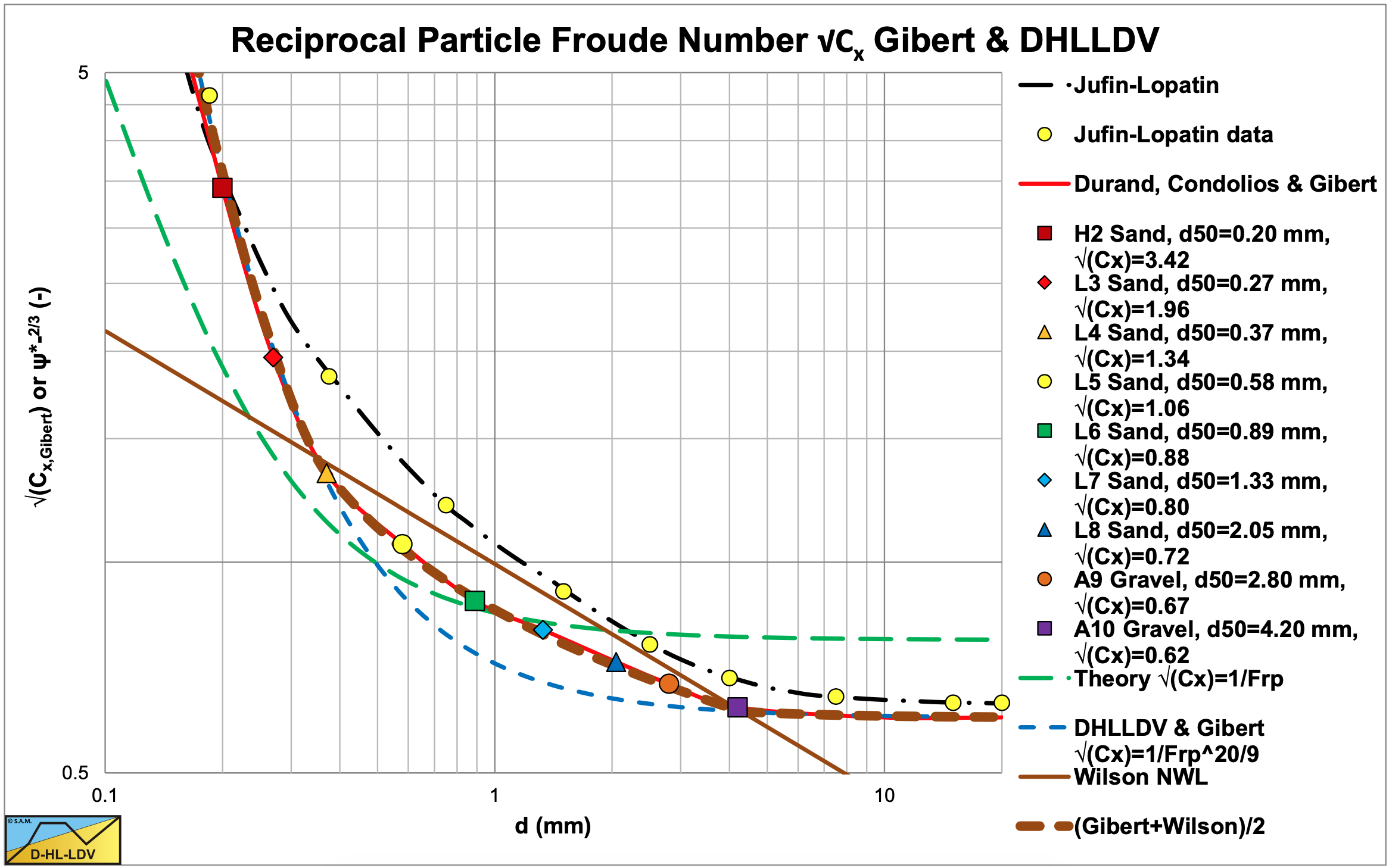
It is also possible to split the particle size distribution into n fraction and determine the weighted average particle Froude number. Gibert (1960) published a graph with values for the particle Froude number that match the findings of Durand & Condolios (1952). Figure 6.4-20 shows these published values. If one uses the values of Gibert (1960), the whole discussion about whether the C_D or the C_x value should be used can be omitted. Analyzing this table however, shows that a very good approximation of the table values can be achieved by using the particle Froude number to the power 20/9 instead of the power 1, assuming that the terminal settling velocity v_t is determined correctly for the solids considered (Stokes, Budryck, Rittinger or Zanke).

\[\ \sqrt{\mathrm{C}_{\mathrm{x}, \mathrm{G i b e r t}}}={\sqrt{\mathrm{C}_{\mathrm{x}}}^{\mathrm{2 0} / \mathrm{9}}}=\mathrm{C}_{\mathrm{x}}^{\mathrm{1 0} / \mathrm{9}}\]

Figure 6.4-20 shows the original data points, the theoretical reciprocal particle Froude numbers using the Zanke (1977) equation for the terminal settling velocity of sand particles and the curve using a power of 20/9. Only for large particles there is a small difference between the original data and the theoretical curve applying the power of 20/9.

Figure 6.4-20: Modified reciprocal particle Froude number, determined experimentally for various sorts of sand and gravel by Durand & Condolios (1952) and Gibert (1960).

6.4.2.1 Inclined Pipes

For inclined pipes they modified the solids effect by adding the cosine of the inclination angle according to:

\[\ \begin{array}{left} \Phi_{\theta}=\frac{\mathrm{i}_{\mathrm{m}, \mathrm{\theta}}-\sin (\theta) \cdot\left(\mathrm{1}+\mathrm{R}_{\mathrm{s d}} \cdot \mathrm{C}_{\mathrm{v t}}\right)-\mathrm{i}_{\mathrm{l}}}{\mathrm{i}_{\mathrm{l}} \cdot \mathrm{C}_{\mathrm{v t}}}=\mathrm{8} \mathrm{1} \cdot\left(\frac{\mathrm{v}_{\mathrm{l}}^{2} \cdot \sqrt{\mathrm{C}_{\mathrm{x}}}}{\mathrm{g} \cdot \mathrm{D}_{\mathrm{p}} \cdot \mathrm{R}_{\mathrm{s d}} \cdot \mathrm{c o s}(\theta)}\right)^{-\mathrm{3} / \mathrm{2}}\\
\mathrm{i}_{\mathrm{m}, \mathrm{\theta}}=\mathrm{i}_{\mathrm{l}} \cdot\left(\mathrm{1}+\mathrm{8 1} \cdot\left(\frac{\mathrm{v}_{\mathrm{l} \mathrm{s}}^{2} \cdot \sqrt{\mathrm{C}_{\mathrm{x}}}}{\mathrm{g} \cdot \mathrm{D}_{\mathrm{p}} \cdot \mathrm{R}_{\mathrm{s d}} \cdot \mathrm{c o s}(\theta)}\right)^{-3 / 2} \cdot \mathrm{C}_{\mathrm{v t}}\right)+\sin (\theta) \cdot\left(\mathrm{1}+\mathrm{R}_{\mathrm{s d}} \cdot \mathrm{C}_{\mathrm{v t}}\right)\end{array}\]

This can be written as:

\[\ \begin{array} \mathrm{i}_{\mathrm{m}, \mathrm{\theta}}=\mathrm{i}_{\mathrm{l}}+\sin (\theta) \cdot\left(\mathrm{1}+\mathrm{R}_{\mathrm{s d}} \cdot \mathrm{C}_{\mathrm{v t}}\right)+\mathrm{i}_{\mathrm{l}} \cdot \mathrm{8 1} \cdot\left(\frac{\mathrm{v}_{\mathrm{l} \mathrm{s}}^{2} \cdot \sqrt{\mathrm{C}_{\mathrm{x}}}}{\mathrm{g} \cdot \mathrm{D}_{\mathrm{p}} \cdot \mathrm{R}_{\mathrm{s d}} \cdot \mathrm{c o s}(\theta)}\right)^{-\mathrm{3} / \mathrm{2}} \cdot \mathrm{C}_{\mathrm{v t}}\\
\mathrm{i}_{\mathrm{m}, \mathrm{\theta}}=\mathrm{i}_{\mathrm{l}, \mathrm{\theta}}+\mathrm{i}_{\mathrm{l}} \cdot \mathrm{8 1} \cdot\left(\frac{\mathrm{v}_{\mathrm{ls}}^{2} \cdot \sqrt{\mathrm{C}_{\mathrm{x}}}}{\mathrm{g} \cdot \mathrm{D}_{\mathrm{p}} \cdot \mathrm{R}_{\mathrm{s d}}}\right)^{-\mathrm{3} / 2} \cdot \mathrm{C}_{\mathrm{v t}} \cdot \cos (\theta)^{3 / 2}+\sin (\theta) \cdot \mathrm{R}_{\mathrm{s d}} \cdot \mathrm{C}_{\mathrm{v} \mathrm{t}}\end{array}\]

So the solids effect has to be multiplied with the cosine of the inclination angle to the power of 3/2. This means the solids effect is decreasing with an increasing inclination angle, whether the inclination is upwards or downwards.

6.4.2.2 The Limit Deposit Velocity

When the flow decreases, there will be a moment where sedimentation of the grains starts to occur. The corresponding line speed is called the Limit Deposit Velocity. Often other terms are used like the critical velocity, critical deposition velocity, deposit velocity, deposition velocity, settling velocity, minimum velocity or suspending velocity. Here we will use the term Limit Deposit Velocity.

Although in literature researchers do not agree on the formulation of the Limit Deposit Velocity, the value of the Limit Deposit Velocity is often derived by differentiating equation (6.4-9) with respect to the line speed v_ls and taking the value of v_ls where the derivative equals zero. This gives:

\[\ \mathrm{v}_{\mathrm{l s}, \mathrm{d v}}=\sqrt{\frac{\mathrm{g} \cdot \mathrm{D}_{\mathrm{p}} \cdot \mathrm{R}_{\mathrm{s d}} \cdot\left(\frac{\mathrm{K} \cdot \mathrm{C}_{\mathrm{v} \mathrm{t}}}{\mathrm{2}}\right)^{2 / 3}}{\sqrt{\mathrm{C}_{\mathrm{x}}}}}\]

At line speeds less than the Limit Deposit Velocity sedimentation occurs and part of the cross-section of the pipe is filled with sand, resulting in a higher flow velocity above the sediment. Durand & Condolios (1952) assume equilibrium between sedimentation and scour, resulting in a Froude number equal to the Froude number at the Limit Deposit Velocity.

\[\ \mathrm{F}_{\mathrm{L}}=\mathrm{F} \mathrm{r}_{\mathrm{l d v}}=\frac{\mathrm{v}_{\mathrm{l s}, \mathrm{d v}}}{\sqrt{\mathrm{g} \cdot \mathrm{D}_{\mathrm{p}} \cdot \mathrm{R}_{\mathrm{s d}}}}=\sqrt{\frac{\left(\frac{\mathrm{K} \cdot \mathrm{C}_{\mathrm{v} \mathrm{t}}}{2}\right)^{2 / 3}}{\sqrt{\mathrm{C}_{\mathrm{x}}}}}\]

By using the hydraulic diameter concept, at lines speeds less than the Limit Deposit Velocity, the resistance can be determined applying equation (6.4-10) using the hydraulic diameter instead of the pipe diameter. At low flows, resulting in small hydraulic diameters, the hydraulic gradient may be so large that a sliding bed may occur, limiting the hydraulic gradient. But Durand & Condolios (1952) did not perform experiments in that flow region. Equation (6.4-15) can be written in the form of the Durand Limit Deposit Velocity based on the minimum pressure loss, according to:

\[\ \begin{array}{left}\mathrm{v}_{\mathrm{l s}, \mathrm{l d v}}=\left(\frac{\mathrm{K} \cdot \mathrm{C}_{\mathrm{v} \mathrm{t}}}{2}\right)^{1 / 3} \cdot \sqrt{\frac{\mathrm{1}}{\mathrm{2} \cdot \sqrt{\mathrm{C}_{\mathrm{x}}}}} {\cdot \sqrt{\mathrm{2 \cdot \mathrm { g } \cdot \mathrm { D } _ { \mathrm { p } , \mathrm { H } } \cdot \mathrm { R } _ { \mathrm { s d } }}}=\mathrm{F}_{\mathrm{L}} \cdot \sqrt{\mathrm{2} \cdot \mathrm{g} \cdot \mathrm{D}_{\mathrm{p}, \mathrm{H}} \cdot \mathrm{R}_{\mathrm{s d}}}}\\
\mathrm{F}_{\mathrm{L}}=\left(\frac{\mathrm{K} \cdot \mathrm{C}_{\mathrm{v} \mathrm{t}}}{\mathrm{2}}\right)^{1 / 3} \cdot \sqrt{\frac{\mathrm{1}}{\mathrm{2} \cdot \sqrt{\mathrm{C}_{\mathrm{x}}}}}\end{array}\]

With minor adjustments for hindered settling and the ratio between the particle size d and the pipe diameter D_p according to Wasp et al. (1970), the following equation is derived by Miedema (1995).

\[\ \mathrm{F_{L}=\left(\frac{K \cdot C_{v t}}{2}\right)^{1 / 3} \cdot \sqrt{\frac{\left(1-C_{v t}\right)^{\beta}}{2 \cdot \sqrt{C_{x}}}} \cdot\left(\frac{1000 \cdot d}{D_{p, H}}\right)^{1 / 6}}\]

The coefficient β is determined with equation (4.6-1). Equation (6.4-18) can be modified to match the original Durand & Condolios (1952) graph according to equation (6.4-19):

\[\ \mathrm{F_{L}=1.9 \cdot\left(\frac{K \cdot C_{v t}}{2}\right)^{1 / 3} \cdot \sqrt{\frac{\left(1-C_{v t}\right)^{\beta}}{2 \cdot \sqrt{C_{x}}}} \cdot\left(\frac{1000 \cdot d}{D_{p, H}}\right)^{1 / 6} \cdot e^{-\frac{d}{0.0006}}+0.6+1.3 \cdot\left(1-e^{-\frac{d}{0.0006}}\right)}\]

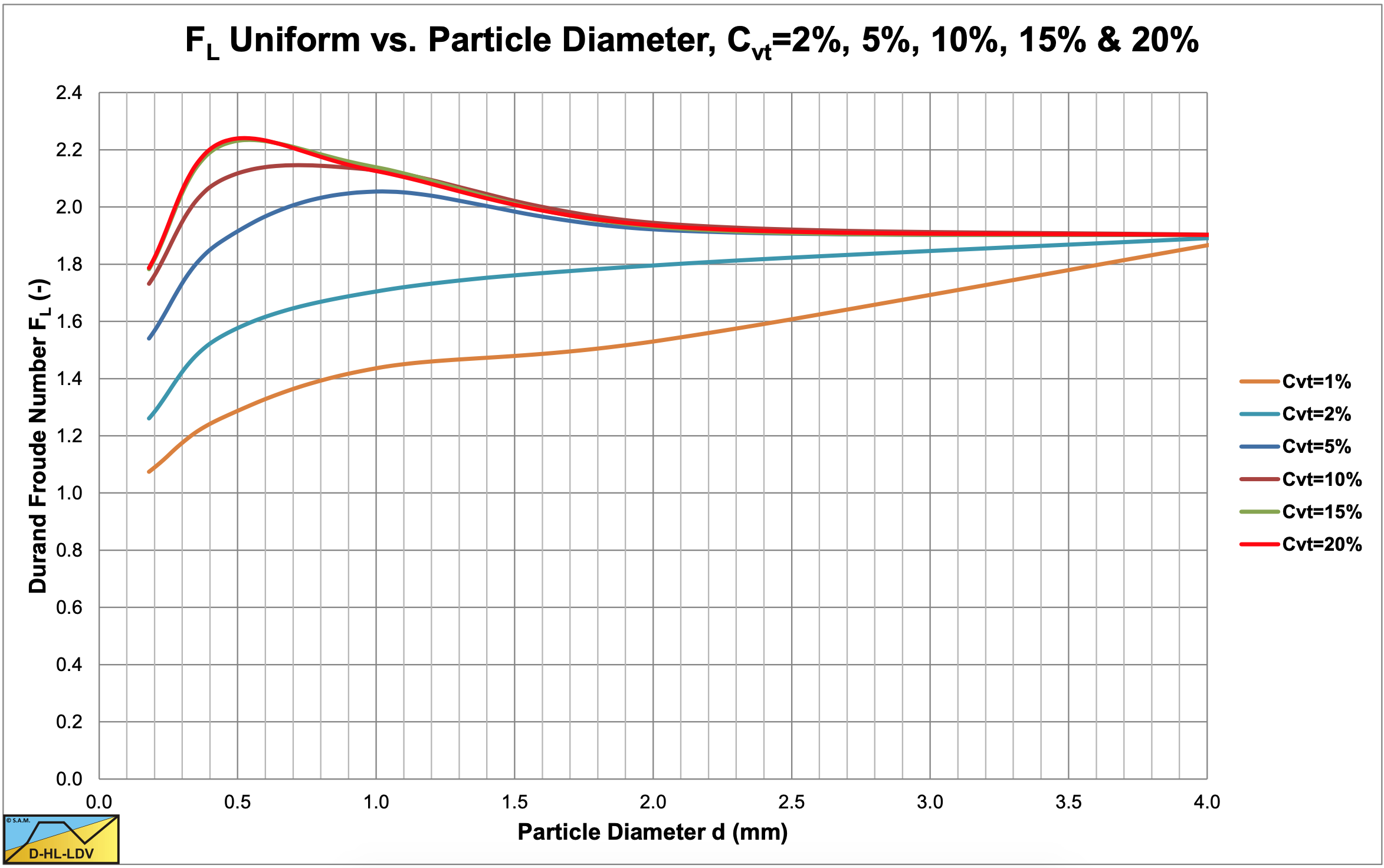
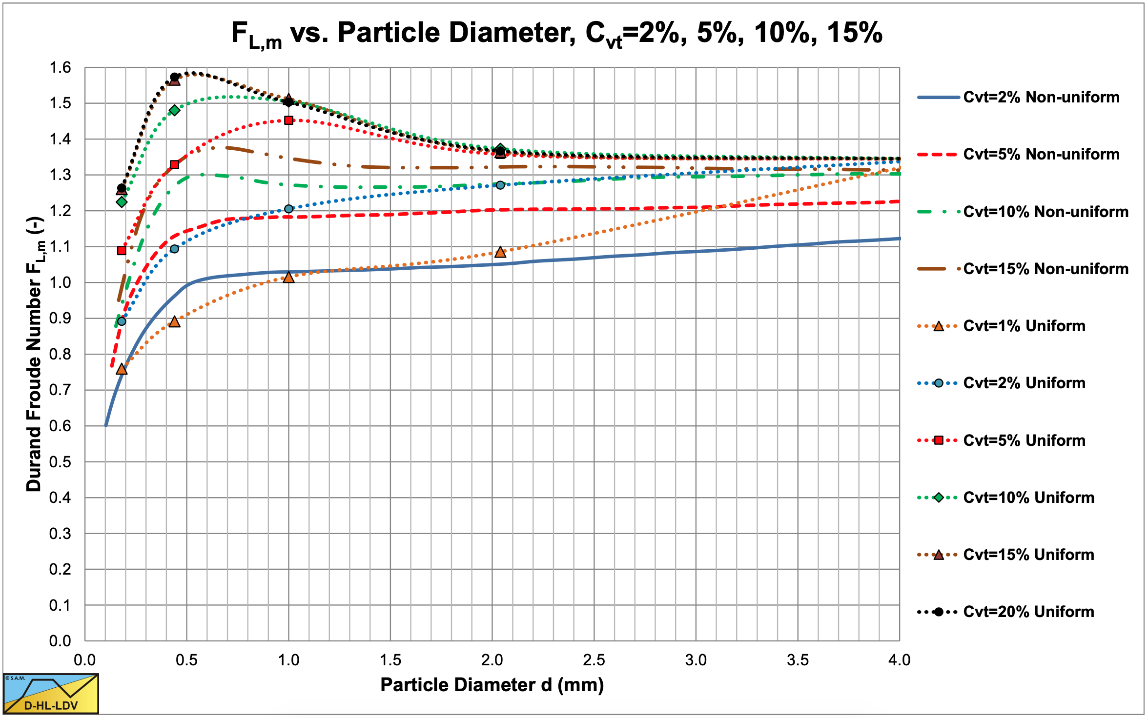
Equation (6.4-19) gives a good approximation of the original F_L graph published by Durand & Condolios (1952). The original graph is shown in Figure 6.4-22, while an approximation for large concentrations is given in Figure 6.4-23. Figure 6.4-24 shows the resulting graph of the modified F_L,m equation (6.4-20). Durand & Condolios (1952) and Gibert used concentrations up to 15% in their graph. Often it is referred to that for higher concentrations the curve of 15% should be used. Figure 6.4-25 shows the curves up to concentrations of 50% according to equation (6.4-20) and shows that for small particle diameters, the value of F_L decreases at the higher concentrations.

\[\ \mathrm{F_{L,m}=\frac{1.9 \cdot (\frac{K \cdot C_{vt}}{2})^{1/3}\cdot \sqrt{\frac{(1-C_{vt})^\beta}{2 \cdot \sqrt{C_x}}}\cdot(\frac{1000 \cdot d}{D_{p, H}})^{1/6} \cdot e^{-\frac{d}{0.0006}}+ 0.6 + 1.3 \cdot(1-e^{-\frac{d}{0.0006}})} {\sqrt{2}}}\]

It should be noted here that Durand & Condolios (1952) did their experiments in medium pipe diameters. The hydraulic gradients in larger pipes are often not high enough to result in a sliding bed. So it is assumed that the Limit Deposit Velocity of Durand & Condolios (1952) is the velocity below which particles are at rest on the bottom of the pipe, forming a stationary bed and not a sliding bed.

Figure 6.4-26 shows the Limit Deposit Velocity, as a function of the pipe diameter D_p and the particle diameter d according to equation (6.4-18), matching the findings of van den Berg (1998). Figure 6.4-27 shows the Limit Deposit Velocity as a function of the pipe diameter D_p and the particle diameter d, according to equation (6.4-19), matching the findings of Durand & Condolios (1952) and Gibert (1960).

Gibert (1960) analyzed the measurements of Durand & Condolios (1952) and created Figure 6.4-21, showing the Froude number F_L at the Limit Deposit Velocity as a function of the volumetric transport concentration C_vt for 5 sands and gravel for pipe diameters D_p of 0.04 m and 0.15 m. He concluded that on average sand H2 has a coefficient F_L=1.7 for higher concentrations, while the other sands and gravel have an F_L=2.1. Tests in a D_p=0.7 m pipeline at concentrations of 15%-20% have resulted in F_L=2.1-2.3. The tendencies found in Figure 6.4-21 confirm the findings of Durand & Condolios (1952), but the asymptotic value of about 1.9 in Figure 6.4-22 and Figure 6.4-23 is a bit low, considering that deposition should be avoided. If we want to predict average behavior, Figure 6.4-24 and Figure 6.4-25 should be used. If we want to prevent deposition at all times, taking into account the scatter, an asymptotic value of about 2.1 should be used, leading to a Limit Deposit Velocity of about 3.3 m/s in a 0.1524 m (6 inch) pipe.

Figure 6.4-21: The Limit Deposit Velocity Froude number F_L as a function of the transport concentration C_vt for 5 different sands and gravel.

Figure 6.4-22: Original Durand coefficient approximation according to equation (6.4-19) (D_p=0.5m) for the original concentrations.

Figure 6.4-23: Original Durand coefficient approximation according to equation (6.4-19) (D_p=0.5m) for large concentrations.

Figure 6.4-24: Modified Durand coefficient approximation according to equation (6.4-20), (D_p=0.5m).

Figure 6.4-25: Modified Durand coefficient approximation according to equation (6.4-20), extrapolated for higher concentrations (D_p=0.5m).

Figure 6.4-26: Limit Deposit Velocity according to equation (6.4-18) at a concentration of 0.1.

Figure 6.4-27: Limit Deposit Velocity according to equation (6.4-19) at a concentration of 0.1.

Figure 6.4-28: The data of Figure 6.4-13 as hydraulic gradient versus line speed.

Figure 6.4-29: The data of Figure 6.4-13 in Durand coordinates.

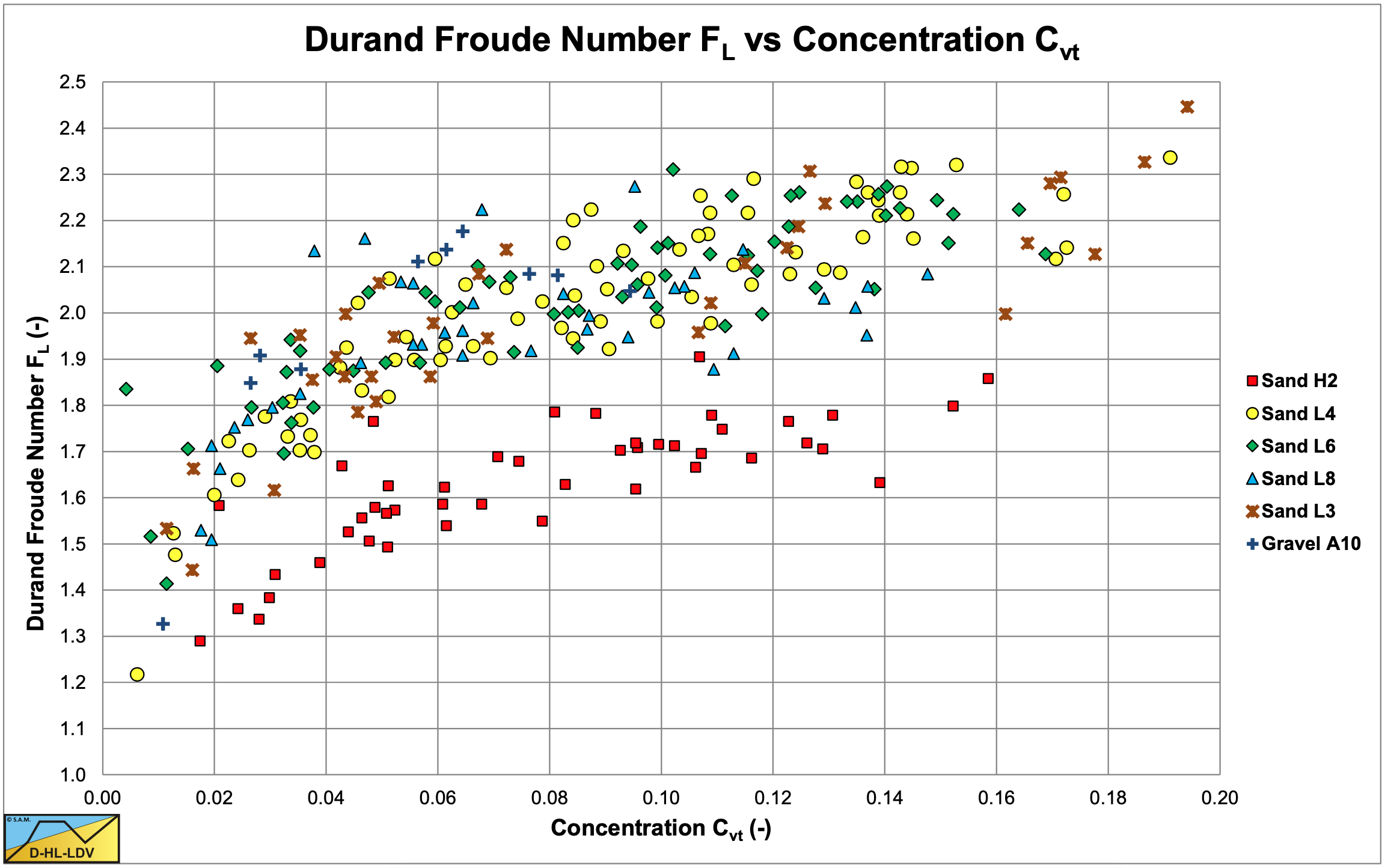
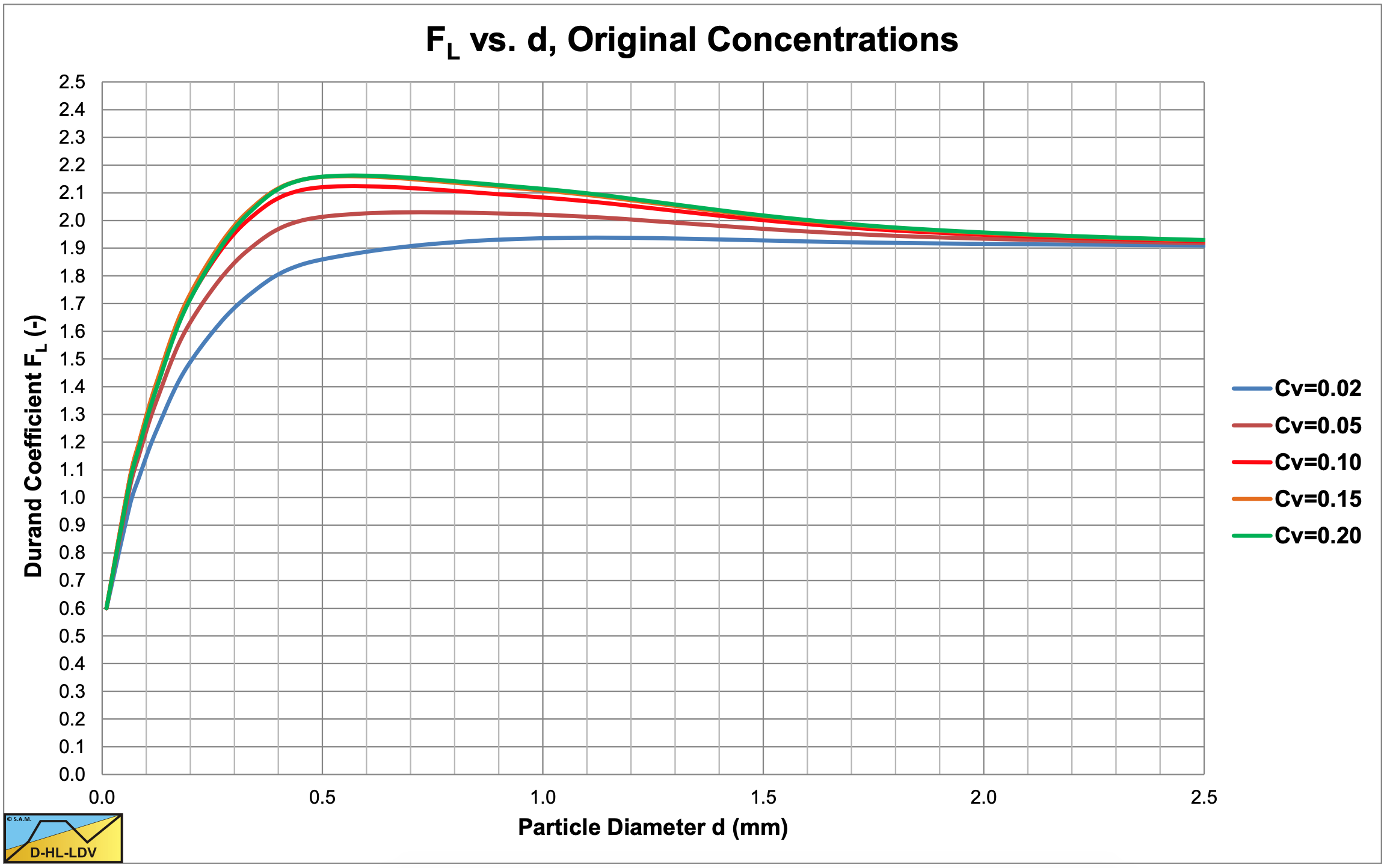
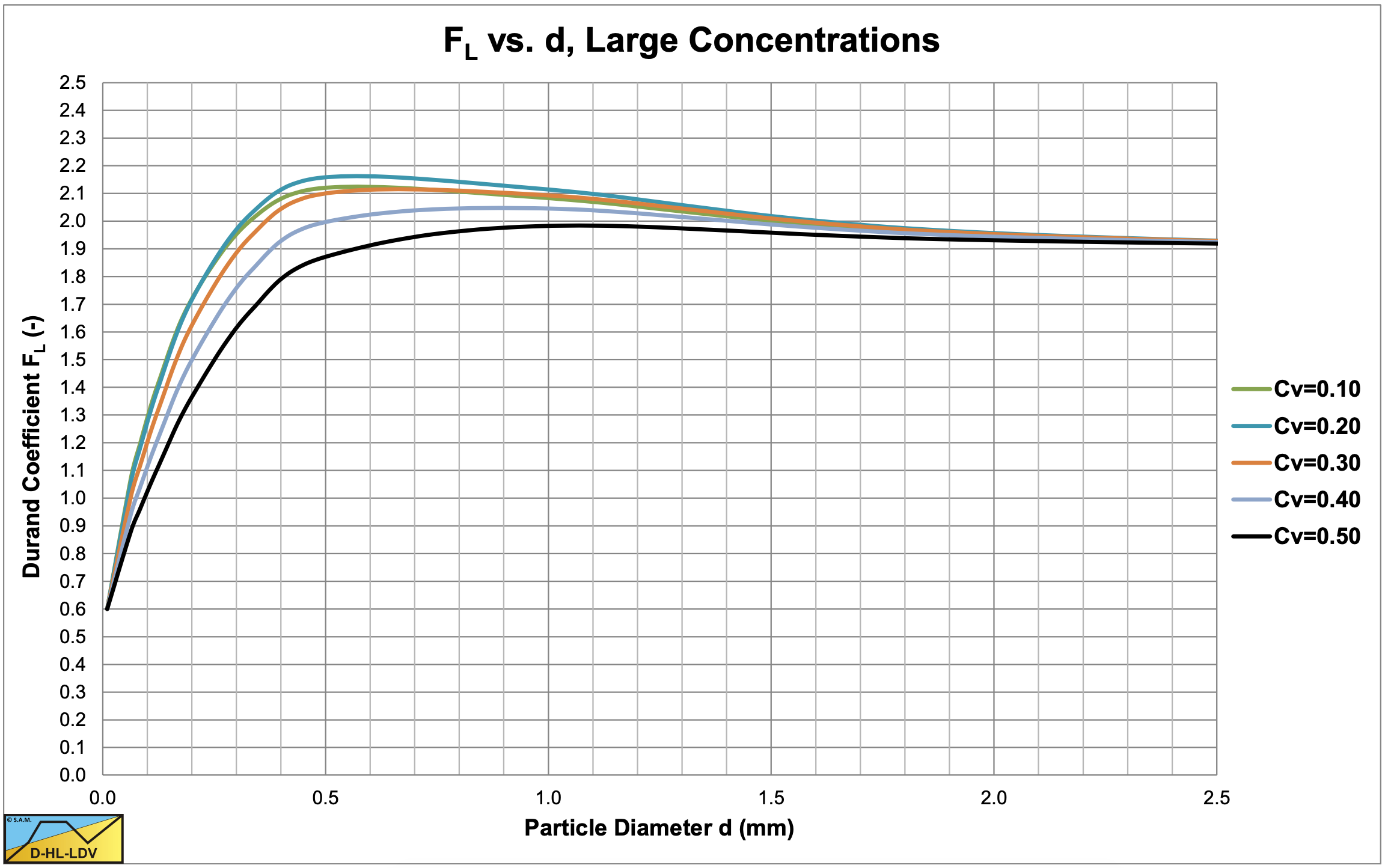
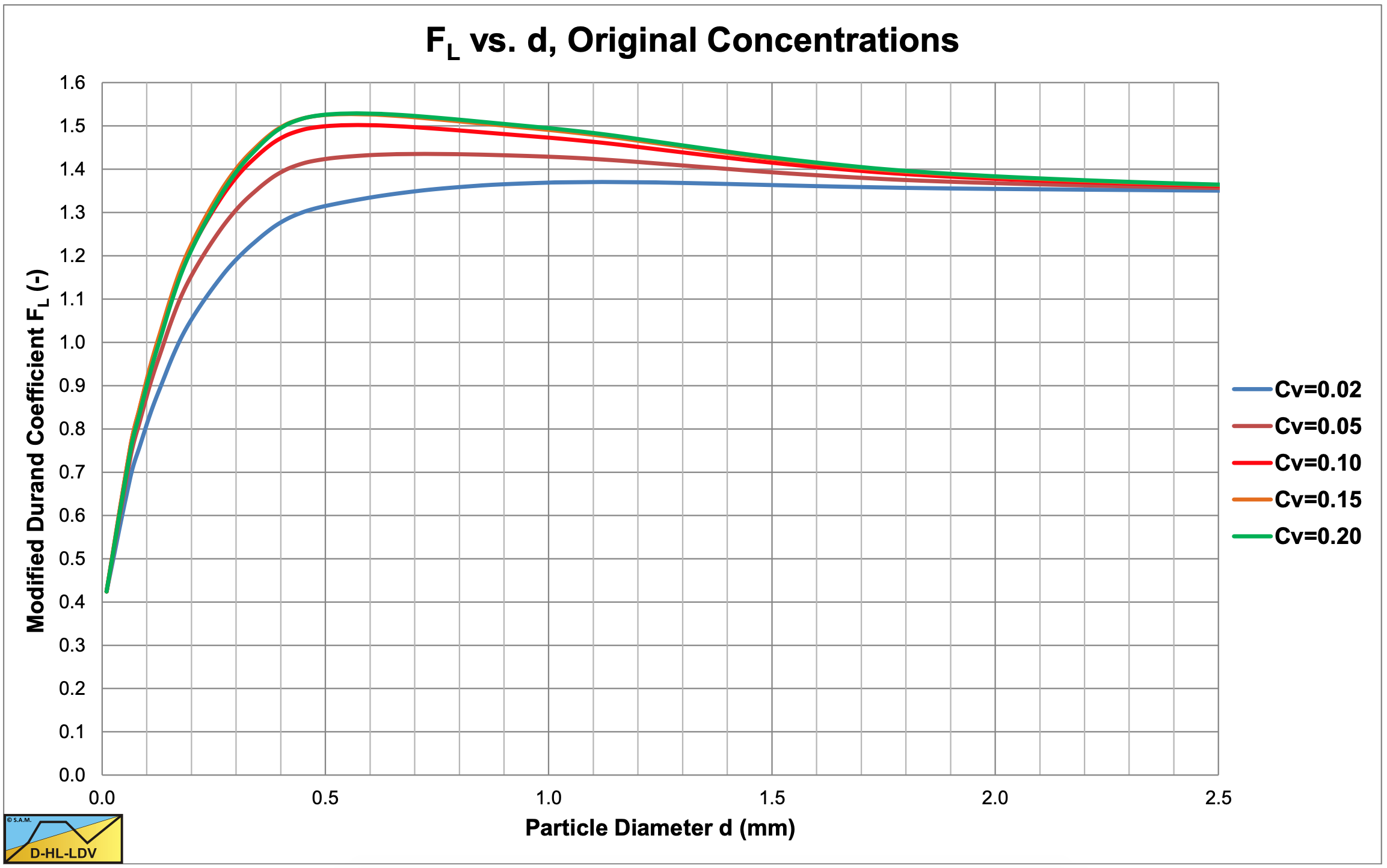
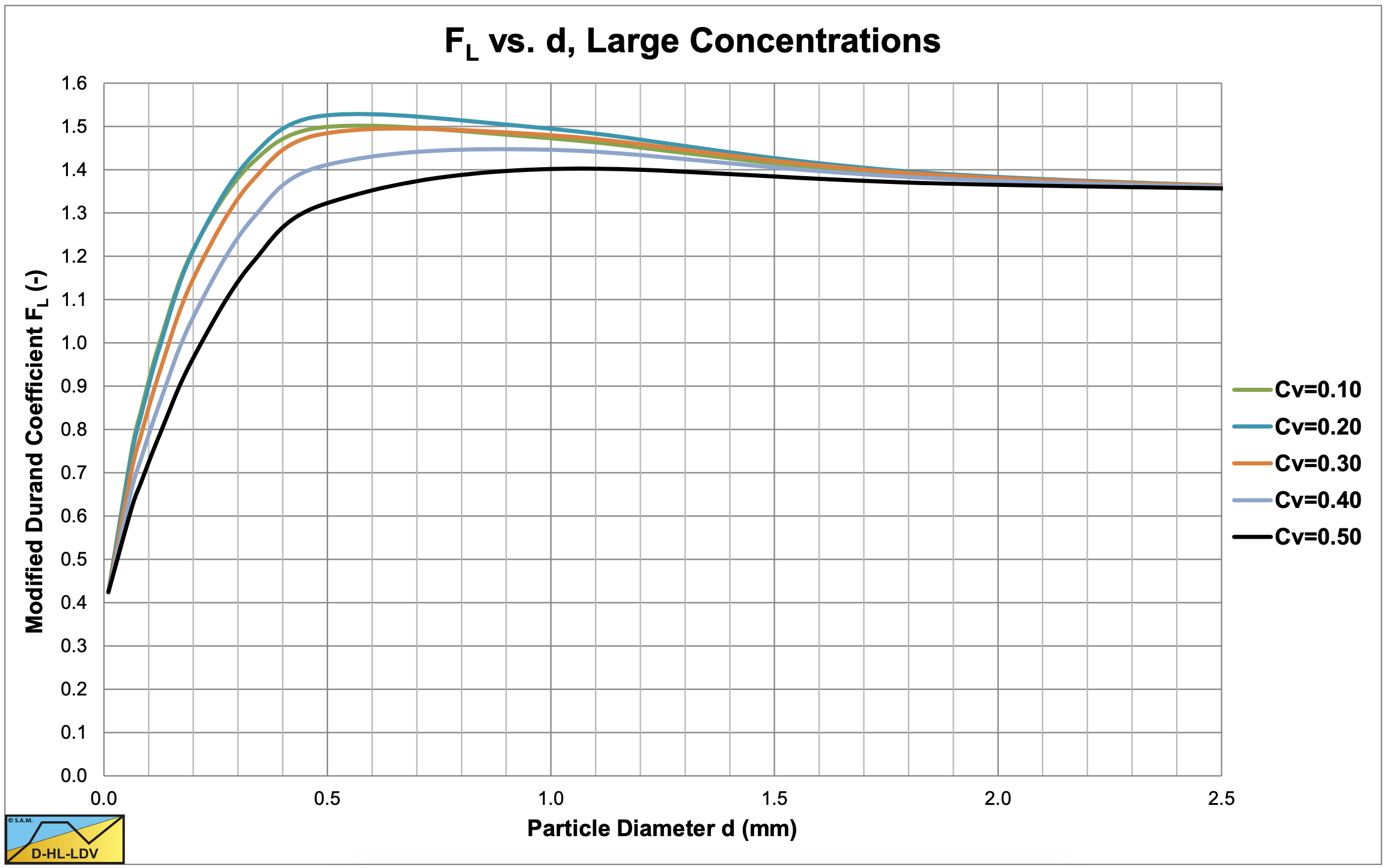
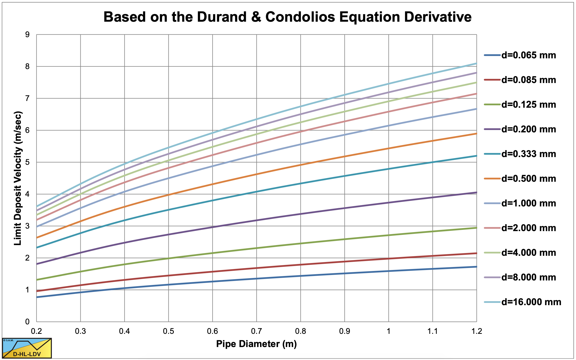
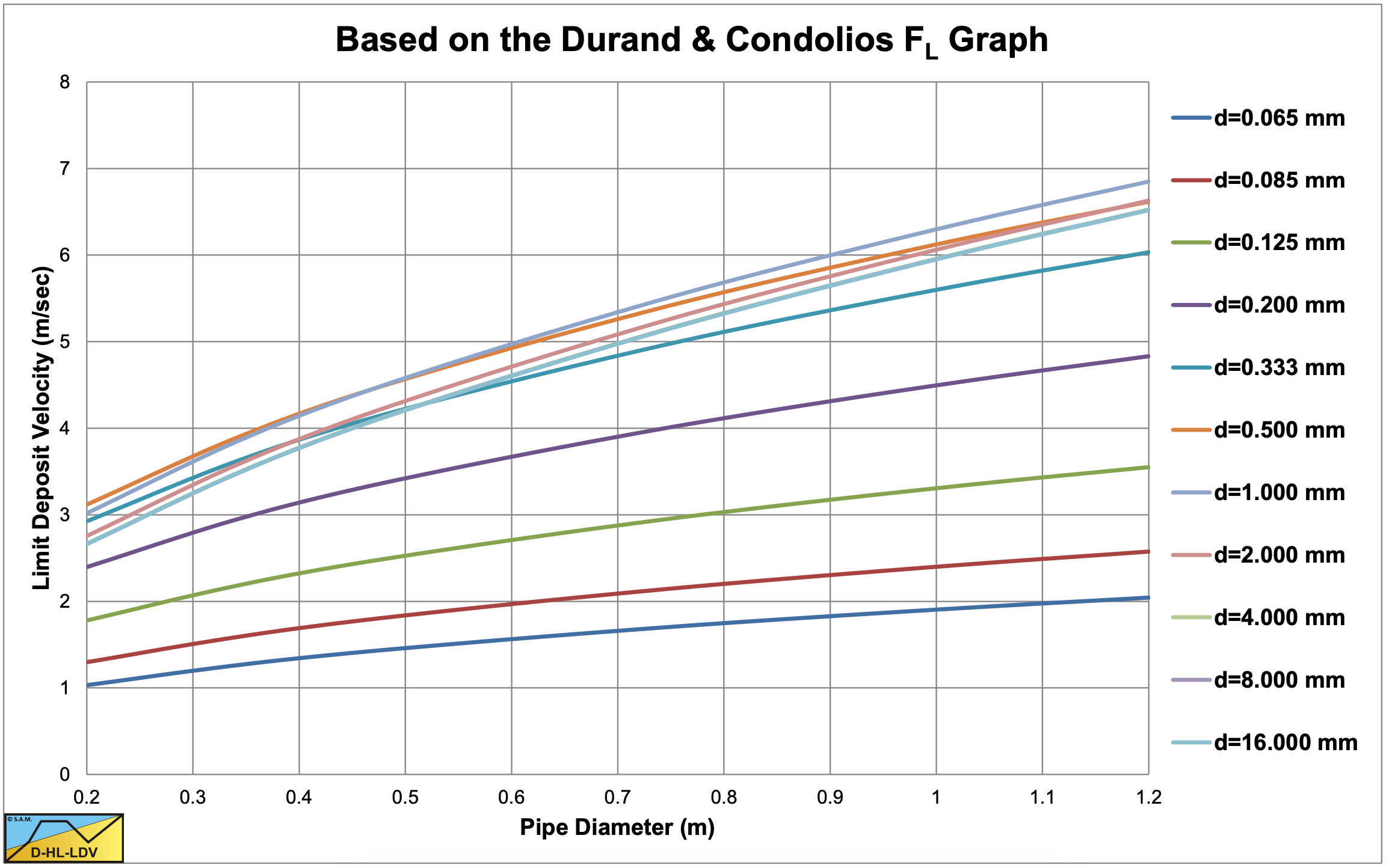
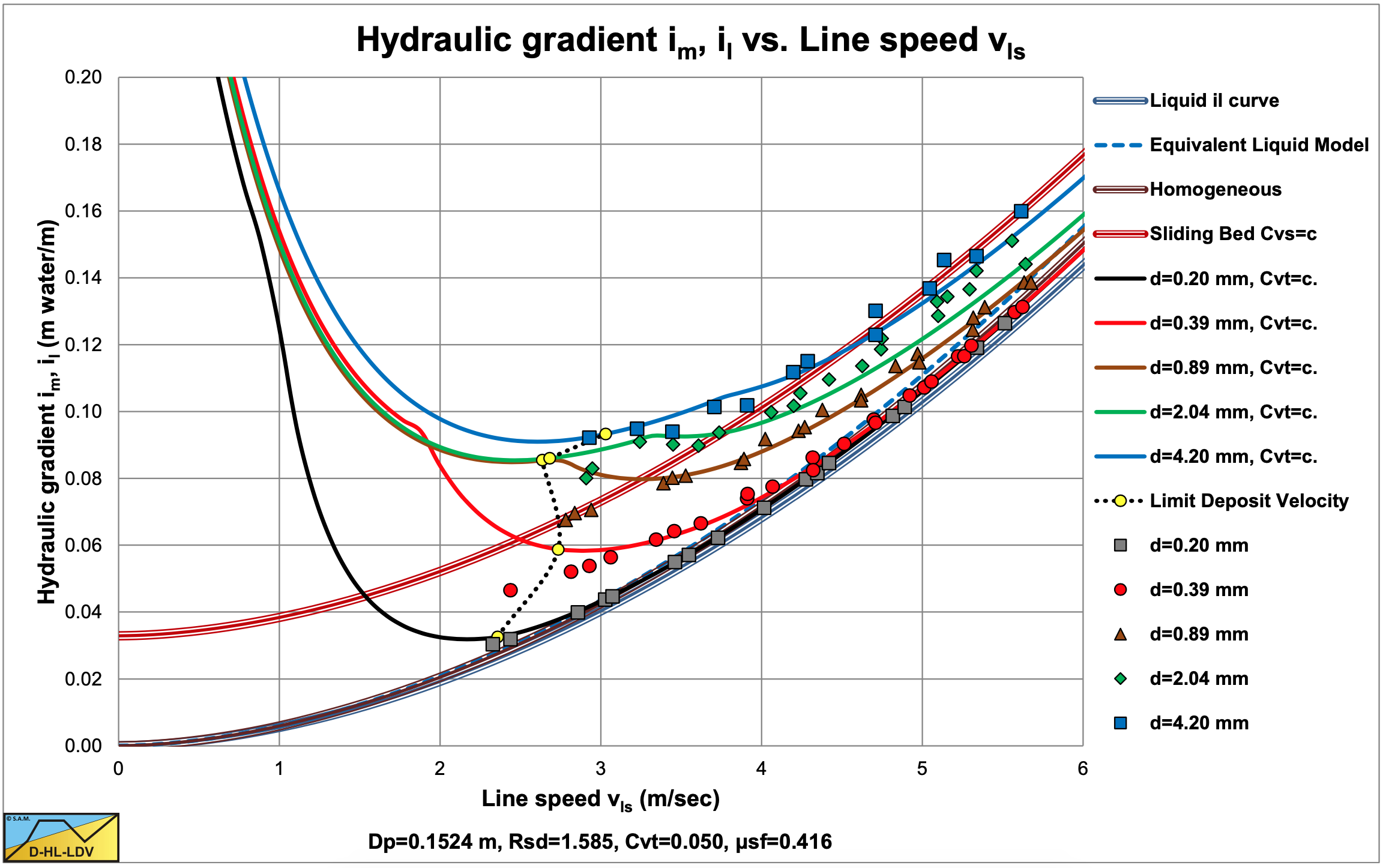
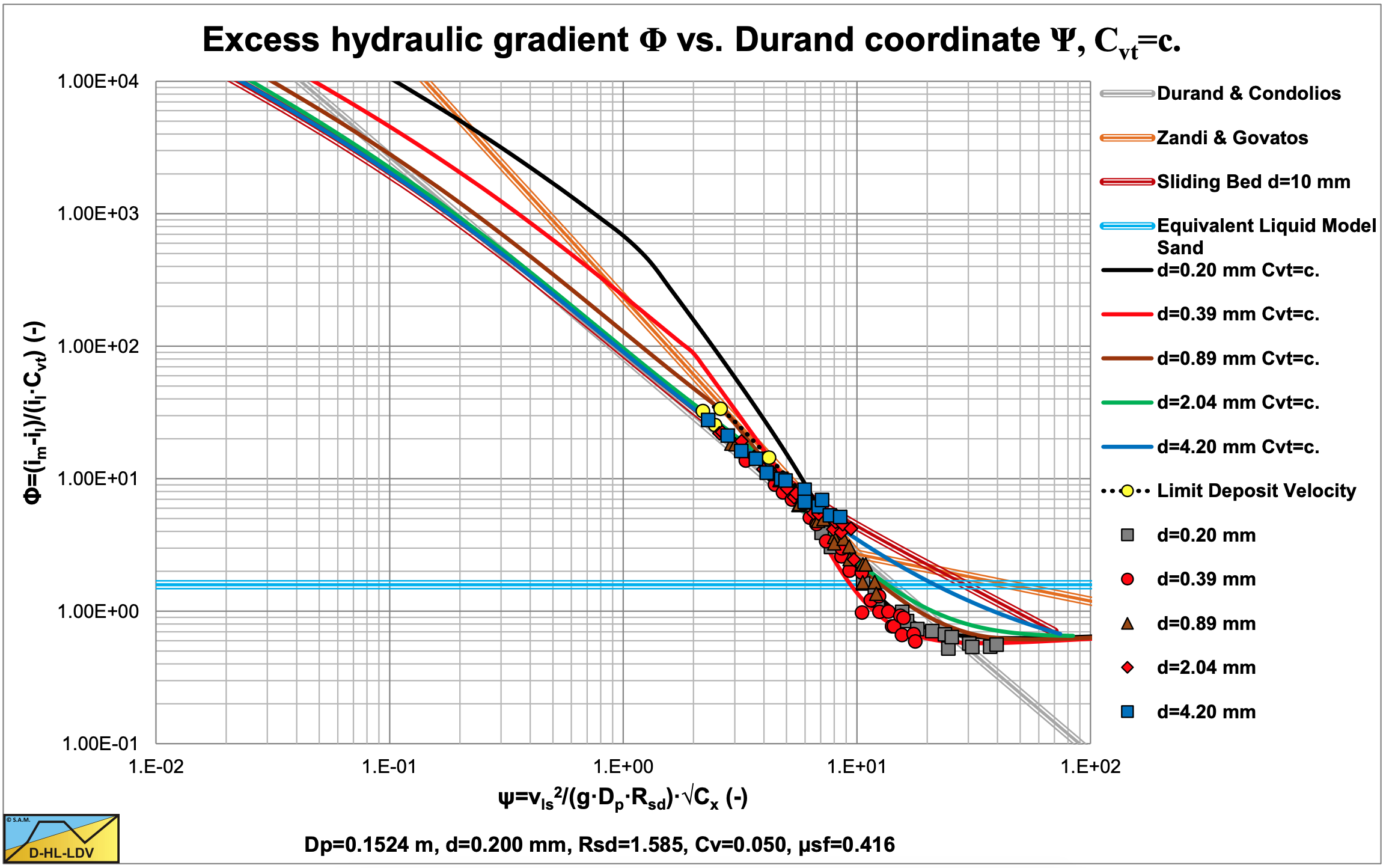
Figure 6.4-28 and Figure 6.4-29 show the data of Figure 6.4-13 in the hydraulic gradient versus line speed graph and in the Durand coordinates graph, normalized for a volumetric concentration of 5%. The solid curves are based on the DHLLDV Framework and match very well.

6.4.3 The Worster & Denny (1955) Model

At about the same time as Durand & Condolios (1952), Worster & Denny (1955) studied flow phenomena of large particles, in particular coal, and produced a similar correlation as Durand & Condolios (1952), except for the inclusion of a term taking into account the specific gravity (relative submerged density) of the solid material and the absence of any parameter of the particle size. In the most general form this equation yields:

\[\ \Delta \mathrm{p}_{\mathrm{m}}=\Delta \mathrm{p}_{\mathrm{l}} \cdot\left(\mathrm{1}+\mathrm{\Phi} \cdot \mathrm{C}_{\mathrm{v}}\right)\]

With:

\[\ \Phi=\frac{\mathrm{i}_{\mathrm{m}}-\mathrm{i}_{\mathrm{l}}}{\mathrm{i}_{\mathrm{l}} \cdot \mathrm{C}_{\mathrm{v}}}=\frac{\Delta \mathrm{p}_{\mathrm{m}}-\Delta \mathrm{p}_{\mathrm{l}}}{\Delta \mathrm{p}_{\mathrm{l}} \cdot \mathrm{C}_{\mathrm{v}}}=\mathrm{1 2 0} \cdot\left(\frac{\mathrm{v}_{\mathrm{l s}}^{2}}{\mathrm{g} \cdot \mathrm{D}_{\mathrm{p}} \cdot \mathrm{R}_{\mathrm{s d}}}\right)^{-\mathrm{3} / 2}\]

Figure 6.4-30 shows the data measured by Worster & Denny (1955) as a function of the Worster parameter ψ.

\[\ \Psi=\left(\frac{\mathrm{v}_{\mathrm{l s}}^{2}}{\mathrm{g} \cdot \mathrm{D}_{\mathrm{p}} \cdot \mathrm{R}_{\mathrm{s d}}}\right)^{\mathrm{1 / 2}}\]

Figure 6.4-30: The data measured by Worster & Denny (1955).

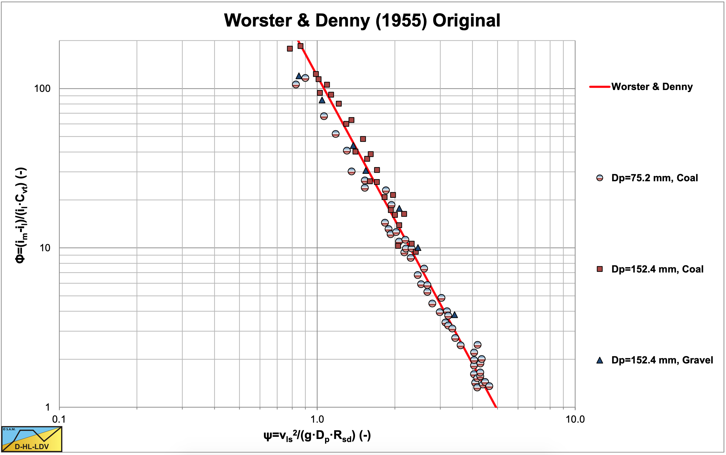
Figure 6.4-31 shows these data as a function of the original Durand parameter ψ, not yet containing the relative submerged density, but containing the particle Froude number √C_x. This parameter is:

\[\ \Psi=\left(\frac{\mathrm{v}_{\mathrm{ls}}^{2}}{\mathrm{g} \cdot \mathrm{D}_{\mathrm{p}}}\right) \cdot \sqrt{\frac{\mathrm{g} \cdot \mathrm{d}}{\mathrm{v}_{\mathrm{t}}^{2}}}=\left(\frac{\mathrm{v}_{\mathrm{l} s}^{2}}{\mathrm{g} \cdot \mathrm{D}_{\mathrm{p}}}\right) \cdot \sqrt{\mathrm{C}_{\mathrm{x}}}\]

Giving the Worster & Denny (1955) equation:

\[\ \Phi=\frac{\mathrm{i}_{\mathrm{m}}-\mathrm{i}_{\mathrm{l}}}{\mathrm{i}_{\mathrm{l}} \cdot \mathrm{C}_{\mathrm{v}}}=\frac{\Delta \mathrm{p}_{\mathrm{m}}-\Delta \mathrm{p}_{\mathrm{l}}}{\Delta \mathrm{p}_{\mathrm{l}} \cdot \mathrm{C}_{\mathrm{v}}}=\mathrm{1 7 2} \cdot \Psi^{-3 / 2}=\mathrm{1 7 2} \cdot\left(\frac{\mathrm{v}_{\mathrm{l} \mathrm{s}}^{2} \cdot \sqrt{\mathrm{C}_{\mathrm{x}}}}{\mathrm{g} \cdot \mathrm{D}_{\mathrm{p}}}\right)^{-3 / 2}\]

Figure 6.4-31: The data of Worster & Denny (1955) in Durand coordinates, without the correction for the relative submerged density R_sd.

Figure 6.4-32: The data of Worster & Denny (1955) in Durand coordinates and corrected for the relative submerged density R_sd.

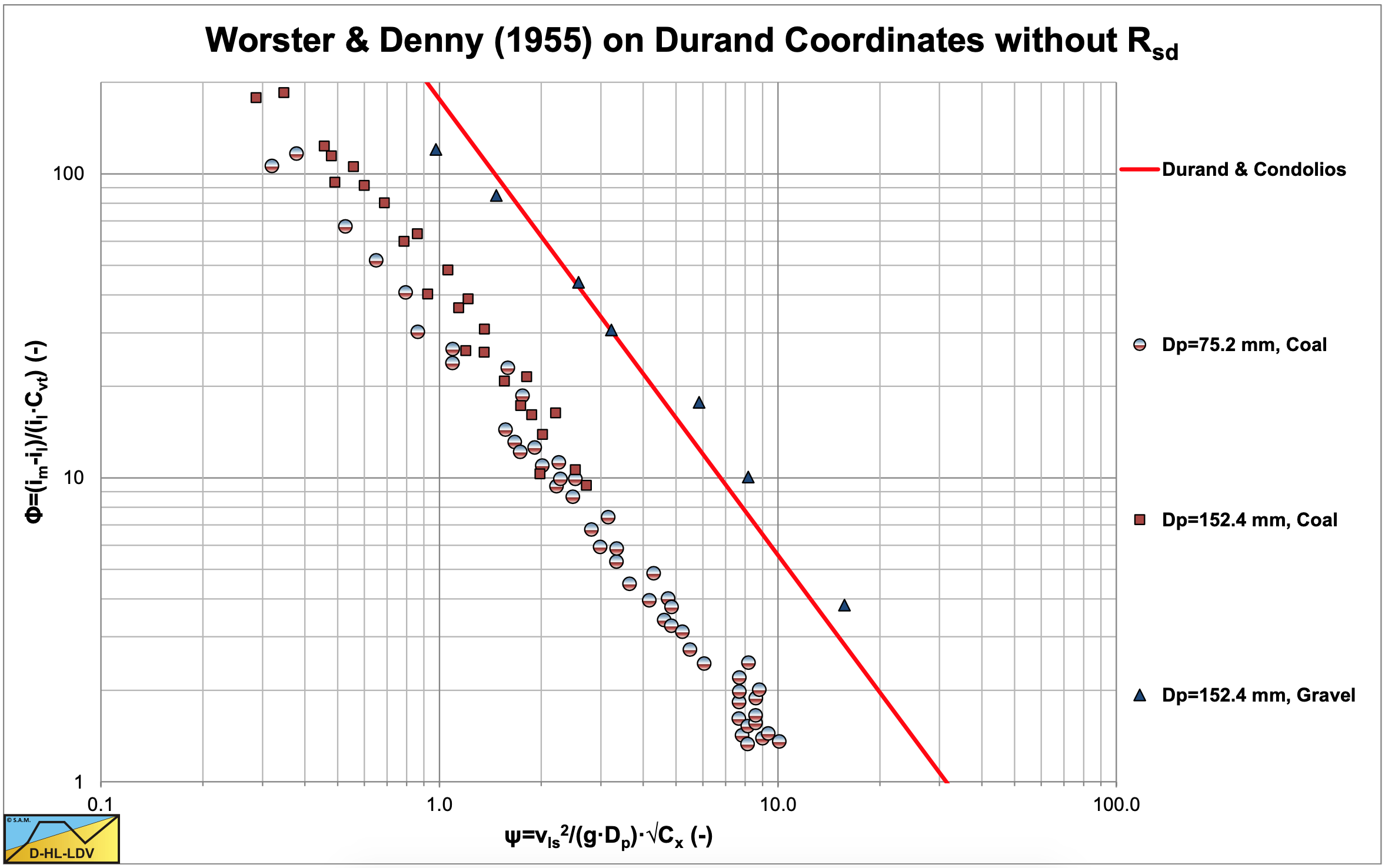
The data points of coal with a relative submerged density different from sand, deviate from the Durand & Condolios (1952) equation as is obvious from Figure 6.4-31. This equation can be modified to make it applicable to materials having a specific gravity different to that of sand and gravel (R_sd =1.65). By taking into account the specific gravity of the solids as Worster & Denny (1955) have done and making the corresponding correction to the constant, using a drag coefficient of 0.4, the following equation is found:

\[\ \Phi=\frac{\mathrm{i}_{\mathrm{m}}-\mathrm{i}_{\mathrm{l}}}{\mathrm{i}_{\mathrm{l}} \cdot \mathrm{C}_{\mathrm{v}}}=\frac{\Delta \mathrm{p}_{\mathrm{m}}-\Delta \mathrm{p}_{\mathrm{l}}}{\Delta \mathrm{p}_{\mathrm{l}} \cdot \mathrm{C}_{\mathrm{v}}}=\mathrm{8} \mathrm{1} \cdot\left(\frac{\mathrm{v}_{\mathrm{l}}^{\mathrm{2}} \cdot \sqrt{\mathrm{C}_{\mathrm{x}}}}{\mathrm{g} \cdot \mathrm{D}_{\mathrm{p}} \cdot \mathrm{R}_{\mathrm{s d}}}\right)^{-3 / 2}\]

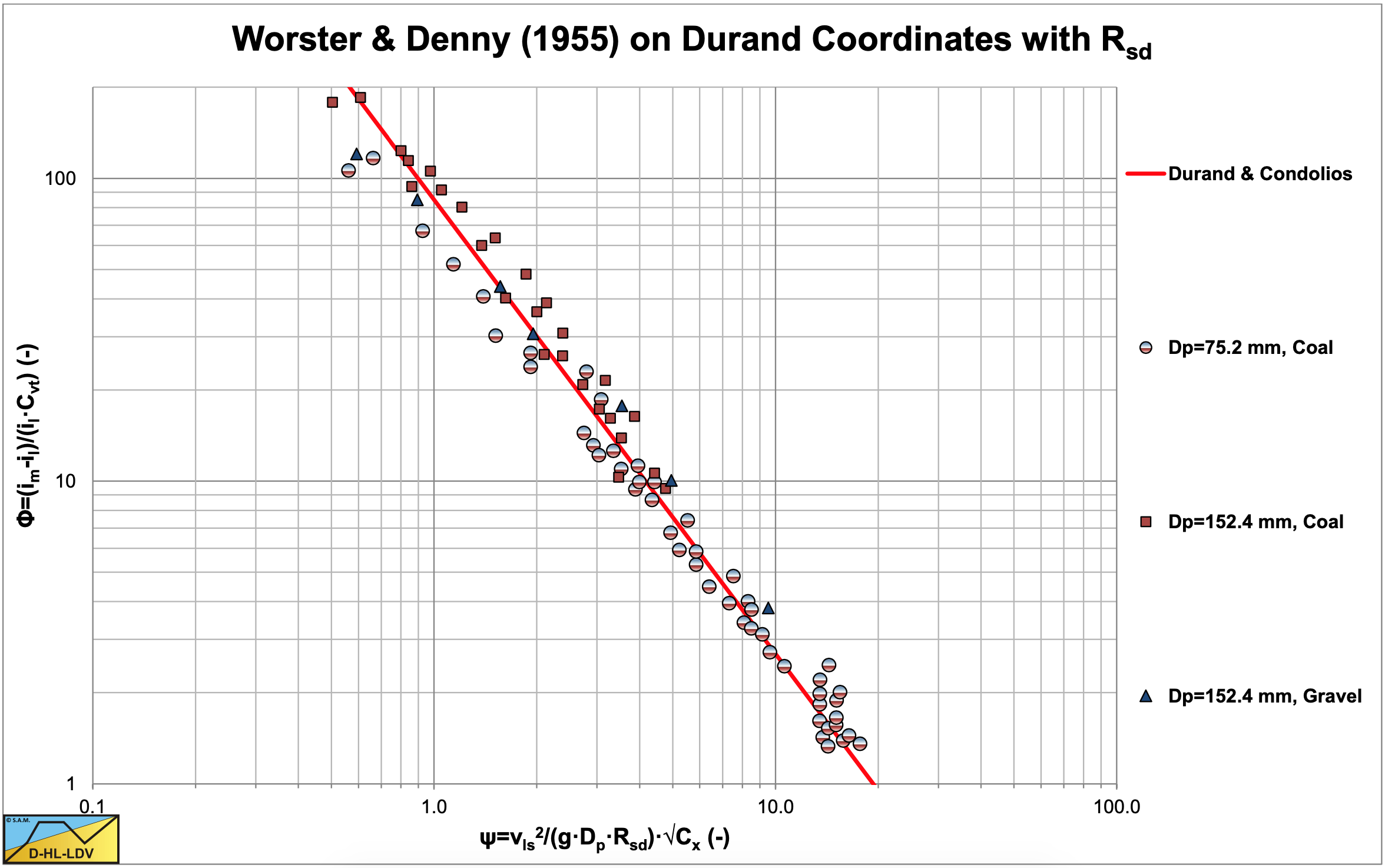
Worster & Denny (1955), estimated the drag coefficient CD for large coal to be 0.4 and changed the coefficient in the above equation from 176/83 to 172/81 to compensate for the relative submerged density (source Bain & Bonnington (1970)). Figure 6.4-32 shows the data of Worster & Denny (1955), as a function of the modified Durand coordinate taking into account the relative submerged density. The data points match the Durand & Condolios (1952) equation very well after the correction for the relative submerged density. Later Gibert (1960) and Condolios & Chapus (1963A) & (1963B) mention the coefficients to be 180/85 instead of 176/83 (Durand & Condolios (1952)) or 172/81 (Worster & Denny (1955)), based on additional experiments. This difference however is marginal and within the scatter of the observations. It should be mentioned that the numbers 180, 176 and 81 are found in literature, while the numbers 85, 83 and 172 are calculated based on a relative submerged density of 1.65. The value of 180 is found in most publications after 1960.

6.4.3.1 Inclined Pipes

Worster & Denny (1955) also gave a method for determining the hydraulic gradient for inclined pipes. Basically the method consists of adding up the pure liquid hydraulic gradient, the potential energy term for the mixture and the solids effect times the cosine of the inclination angle.

For pure liquid the hydraulic gradient in an inclined pipe equals the hydraulic gradient in a horizontal pipe of the same length plus the potential energy, giving:

\[\ \mathrm{i}_{\mathrm{l}, \mathrm{\theta}}=\mathrm{i}_{\mathrm{l}}+\sin (\boldsymbol{\theta})\]

Including the solids effect this gives:

\[\ \mathrm{i}_{\mathrm{m}, \mathrm{\theta}}=\mathrm{i}_{\mathrm{l}, \mathrm{\theta}}+\left(\mathrm{i}_{\mathrm{m}}-\mathrm{i}_{\mathrm{l}}\right) \cdot \cos (\theta)+\mathrm{R}_{\mathrm{s d}} \cdot \mathrm{C}_{\mathrm{v} \mathrm{s}} \cdot \sin (\theta)\]

Using the relative solids effect, the relative excess hydraulic gradient, this can be written as:

\[\ \mathrm{i}_{\mathrm{m}, \mathrm{\theta}}=\mathrm{i}_{\mathrm{l}, \mathrm{\theta}}+\mathrm{E}_{\mathrm{r h g}} \cdot \mathrm{R}_{\mathrm{s d}} \cdot \mathrm{C}_{\mathrm{v s}} \cdot \mathrm{c o s}(\boldsymbol{\theta})+\mathrm{R}_{\mathrm{s d}} \cdot \mathrm{C}_{\mathrm{v s}} \cdot \sin (\boldsymbol{\theta})\]

This can also be written as:

\[\ \mathrm{i}_{\mathrm{m}, \mathrm{\theta}}=\mathrm{i}_{\mathrm{l}}+\mathrm{E}_{\mathrm{r h g}} \cdot \mathrm{R}_{\mathrm{s d}} \cdot \mathrm{C}_{\mathrm{v s}} \cdot \cos (\theta)+\left(\mathrm{1}+\mathrm{R}_{\mathrm{s d}} \cdot \mathrm{C}_{\mathrm{v s}}\right) \cdot \sin (\mathrm{\theta})\]

The relative excess hydraulic gradient of an inclined pipe is now:

\[\ \mathrm{E}_{\mathrm{rhg}, \theta}=\frac{\mathrm{i}_{\mathrm{m}, \theta}-\mathrm{i}_{\mathrm{l}, \theta}}{\mathrm{R}_{\mathrm{s d}} \cdot \mathrm{C}_{\mathrm{v s}}}=\mathrm{E}_{\mathrm{r h g}} \cdot \cos (\theta)+\sin (\theta)\]

This means that the hydraulic gradient of the mixture, excluding the potential energy term, decreases with the cosine of the inclination angle. Both for ascending and descending pipes. It is the question whether this is true for all flow regimes. Different flow regimes may respond differently to the pipe inclination angle. For a vertical pipe this would mean that the solids effect becomes zero, which is questionable. At least for very small particles, following the equivalent liquid model, it is expected that this will not change because of an inclination angle.

Durand & Condolios (1952) found a power of 3/2 for the cosine of the inclination angle.

6.4.4 The Zandi & Govatos (1967) Model

Zandi and Govatos (1967) and later Zandi (1971) extended the work of Durand & Condolios (1952) and later Gibert (1960) to other solids and different mixtures. They used a computer and attempted to assess the validity of the Durand & Condolios (1952) correlation in respect of over 2500 data points from a number of sources, covering a wide range of values of all relevant parameters. They conclude that the Durand & Condolios (1952) expression is totally invalid for solids transported by saltation or sliding bed, although their published evidence (Figure 6.4-33) points in another direction. For heterogeneous transport they claim that the available data are more accurately correlated by two expressions (equations (6.4-34) and (6.4-35)).

They defined a non-dimensionless number to characterize the separation of the flow regime, from saltating/sliding bed to heterogeneous suspension:

\[\ \mathrm{N}_{\mathrm{cr}}=\frac{\mathrm{v}_{\mathrm{l s}}^{2} \cdot \sqrt{\mathrm{C}_{\mathrm{D}}}}{\mathrm{g} \cdot \mathrm{R}_{\mathrm{s d}} \cdot \mathrm{D}_{\mathrm{p}} \cdot \mathrm{C}_{\mathrm{v} \mathrm{t}}}\]

They state that at a critical value of N_cr=40 the transition between a saltating and a heterogeneous regime occurs. This means that at values below 40 a saltating regime occurs and at values equal to or larger than 40 a heterogeneous flow develops. Babcock (1970) analyzed the work of Zandi & Govatos (1967) and concluded that for graded fine particles the transition already may occur at an index number of 10 instead of 40. Complex mixtures with particles of different sizes may increase the index number. No suggestions are offered for an improved correlation for the saltating/sliding bed flow regime.

Zandi & Govatos (1967) based their results on experiments (2500 data points) on sand with particles up to 25 mm, pipe diameters ranging from 0.0375 m to 0.55 m and volumetric concentrations up to 22%. They introduced a second index, which in fact is the Durand abscissa:

\[\ \Psi=\mathrm{C}_{\mathrm{v} \mathrm{t}} \cdot \mathrm{N}_{\mathrm{c r}}=\frac{\mathrm{v}_{\mathrm{l} \mathrm{s}}^{2} \cdot \sqrt{\mathrm{C}_{\mathrm{D}}}}{\mathrm{g} \cdot \mathrm{R}_{\mathrm{s d}} \cdot \mathrm{D}_{\mathrm{p}}}::\left(\frac{\mathrm{v}_{\mathrm{l} s}^{2}}{\mathrm{g} \cdot \mathrm{D}_{\mathrm{p}} \cdot \mathrm{R}_{\mathrm{s d}}}\right) \cdot \sqrt{\frac{\mathrm{g} \cdot \mathrm{d}}{\mathrm{v}_{\mathrm{t}}^{2}}}=\left(\frac{\mathrm{v}_{\mathrm{l} s}^{2}}{\mathrm{g} \cdot \mathrm{D}_{\mathrm{p}} \cdot \mathrm{R}_{\mathrm{s d}}}\right) \cdot \sqrt{\mathrm{C}_{\mathrm{x}}}\]

Zandi & Govatos (1967) use a modified Durand parameter with C_D instead of C_x. At a value of ψ=10 they found a dramatic change in behavior of the pressure losses. Below the value of ψ=10 for real heterogeneous transport they found:

\[\ \Delta \mathrm{p}_{\mathrm{m}}=\Delta \mathrm{p}_{\mathrm{l}} \cdot\left(\mathrm{1}+\mathrm{2} \mathrm{8} \mathrm{0} \cdot \Psi^{-\mathrm{1} . \mathrm{9 3}} \cdot \mathrm{C}_{\mathrm{v t}}\right)\]

Above the value of ψ=10 as a transition between heterogeneous and homogeneous transport they found:

\[\ \Delta \mathrm{p}_{\mathrm{m}}=\Delta \mathrm{p}_{\mathrm{l}} \cdot\left(\mathrm{1}+\mathrm{6} . \mathrm{3} \cdot \Psi^{-\mathrm{0 . 3 5 4}} \cdot \mathrm{C}_{\mathrm{v t}}\right)\]

Based on equation (6.4-33) N_cr=40, a Limit Deposit Velocity can be defined:

\[\ \mathrm{v}_{\mathrm{l s}, \mathrm{l d v}}=\sqrt{\frac{\mathrm{4 0 \cdot g \cdot R}_{\mathrm{s d}} \cdot \mathrm{D}_{\mathrm{p}} \cdot \mathrm{C}_{\mathrm{v t}}}{\sqrt{\mathrm{C}_{\mathrm{D}}}}}\]

Figure 6.4-33 shows the Zandi & Govatos (1967) fit relations together with the Durand & Condolios (1952) and Gibert relation. From the measurements as shown in this figure it is not obvious which relation is the best and whether it should be straight lines. The intersection point where the equations (6.4-34) and (6.4-35) intersect is not exactly 10 but 11.1. This intersection point may be considered the transition between heterogeneous and pseudo homogeneous transport. The critical value of N_cr=40, above which the transport is supposed to be heterogeneous, is difficult to apply and does not match the 2 equations of Zandi & Govatos (1967).

The main value of the work of Zandi & Govatos (1967) lies in recognizing a criterion to differentiate between the saltating/sliding bed regime and the heterogeneous regime. The assertion that the data correlation of Durand & Condolios (1952) is invalid in the case of saltation/sliding bed transport, cannot be accepted based on the evidence in Figure 6.4-33, where remarkably close grouping of the data points with N_cr<40 is found, around the mean curve of Durand & Condolios (1952), from which their correlation was deduced.

Figure 6.4-33: The Zandi & Govatos (1967) fits for heterogeneous slurry flow.

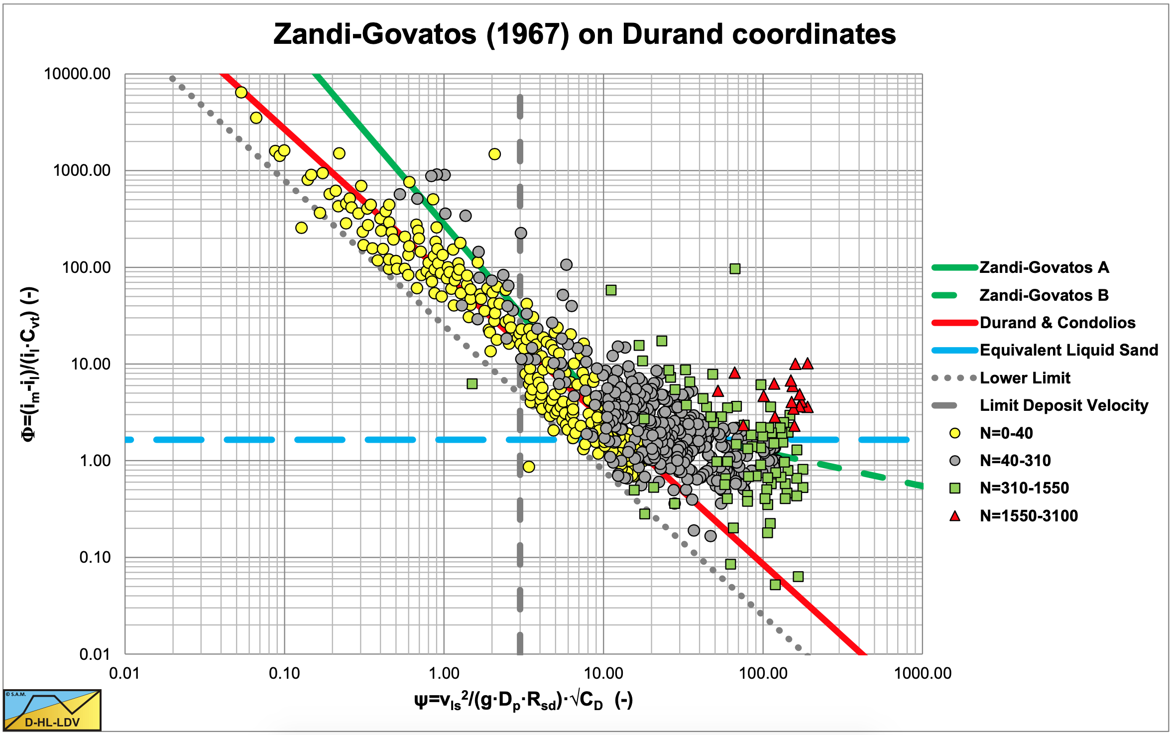
The data points are digitized from a graph of Wilson (1992) (Fig. 3.2) and are not too accurate. The tendencies however are clear. The horizontal coordinate is the modified Durand coordinate, including the submerged relative density. It should be noted that in the original graph, the Durand and the lower Zandi & Govatos (1967) lines were not drawn correctly. For the drag coefficient in the horizontal coordinate, the particle Froude number is assumed as used by Durand & Condolios (1952) & Gibert (1960). The Durand & Condolios (1952) and Gibert (1960) line is drawn with a constant of 85. The lower limit line has a constant of 25. The critical velocity line is the line for very coarse particles, having a particle Froude number of about 0.8, according to Durand & Condolios (1952) and Gibert (1960). Figure 6.4-33 & Figure 6.4-34 show the solutions of Durand & Condolios (1952) and Gibert (1960), Zandi & Govatos (1967) in a correct way. It seems like Zandi & Govatos (1967) focused on the ψ axis when they concluded a ψ=10 is a transition between two physical processes. However they should have focused on the Φ axis where a Φ= R_sd represents the equivalent liquid model or pseudo homogeneous flow. It should also be noted that the power M=1.7 for very narrow graded sands of Wilson et al. (1997), resulting in a power of -3.7 of the line speed in the Durand coordinates, matches the power of -1.93 of Zandi & Govatos (1967), resulting in a power of -3.86 of the line speed in the Durand coordinates, closely.

Considering a Limit Deposit Velocity of (using the limit F_L=1.34 for large particles):

\[\ \mathrm{v}_{\mathrm{l s}, \mathrm{d v}}=\mathrm{F}_{\mathrm{L}} \cdot \sqrt{\mathrm{2} \cdot \mathrm{g} \cdot \mathrm{D}_{\mathrm{p}} \cdot \mathrm{R}_{\mathrm{s d}}} \approx \mathrm{1 . 3 4} \cdot \sqrt{\mathrm{2} \cdot \mathrm{g} \cdot \mathrm{D}_{\mathrm{p}} \cdot \mathrm{R}_{\mathrm{s d}}}\]

And:

\[\ \Psi=\frac{\mathrm{v}_{\mathrm{l s}, \mathrm{ldv}}^{\mathrm{2}}}{\mathrm{g} \cdot \mathrm{D}_{\mathrm{p}}} \cdot \frac{\sqrt{\mathrm{C}_{\mathrm{x}}}}{\mathrm{R}_{\mathrm{s d}}}\]

This gives:

\[\ \Psi=\frac{\mathrm{F}_{\mathrm{L}}^{2} \cdot \mathrm{2} \cdot \mathrm{g} \cdot \mathrm{D}_{\mathrm{p}} \cdot \mathrm{R}_{\mathrm{s} \mathrm{d}}}{\mathrm{g} \cdot \mathrm{D}_{\mathrm{p}}} \cdot \frac{\sqrt{\mathrm{C}_{\mathrm{x}}}}{\mathrm{R}_{\mathrm{s d}}}=\mathrm{2} \cdot \mathrm{F}_{\mathrm{L}}^{2} \cdot \sqrt{\mathrm{C}_{\mathrm{x}}}=2 \cdot \mathrm{1 . 3 4}^{2} \cdot \mathrm{0} . \mathrm{8}=\mathrm{2 . 8 7}\]

For very fine particles, the particle Froude number may be near a value of 5, resulting in a ψ of almost 18 for sand. For coal with a relative submerged density of 0.4-0.6 the values can be higher.
It is remarkable that at the lower limit of the Limit Deposit Velocity of about 3, there is a sort of limit in the data points.

It should also be mentioned that the Durand & Condolios (1952) and Gibert (1960) line match data points in the heterogeneous regime, but also in the sliding bed/saltation regime. The two lines of Zandi & Govatos (1967) match the heterogeneous regime (upper line) and the transition heterogeneous/pseudo homogeneous (lower line). The fact that many points are below the pseudo homogeneous line for sand, has two reasons. First of all, the location of this line depends on the relative submerged density of the solids, so for coal it will be 0.4-0.6, while for aluminum it will be 2.65. The second reason is that in many cases there is some overshoot; higher velocities are required to reach the pseudo homogeneous regime.

Figure 6.4-34: The Durand & Condolios (1952), Gibert (1960), and Zandi & Govatos (1967) solutions on Durand coordinates, zoomed.

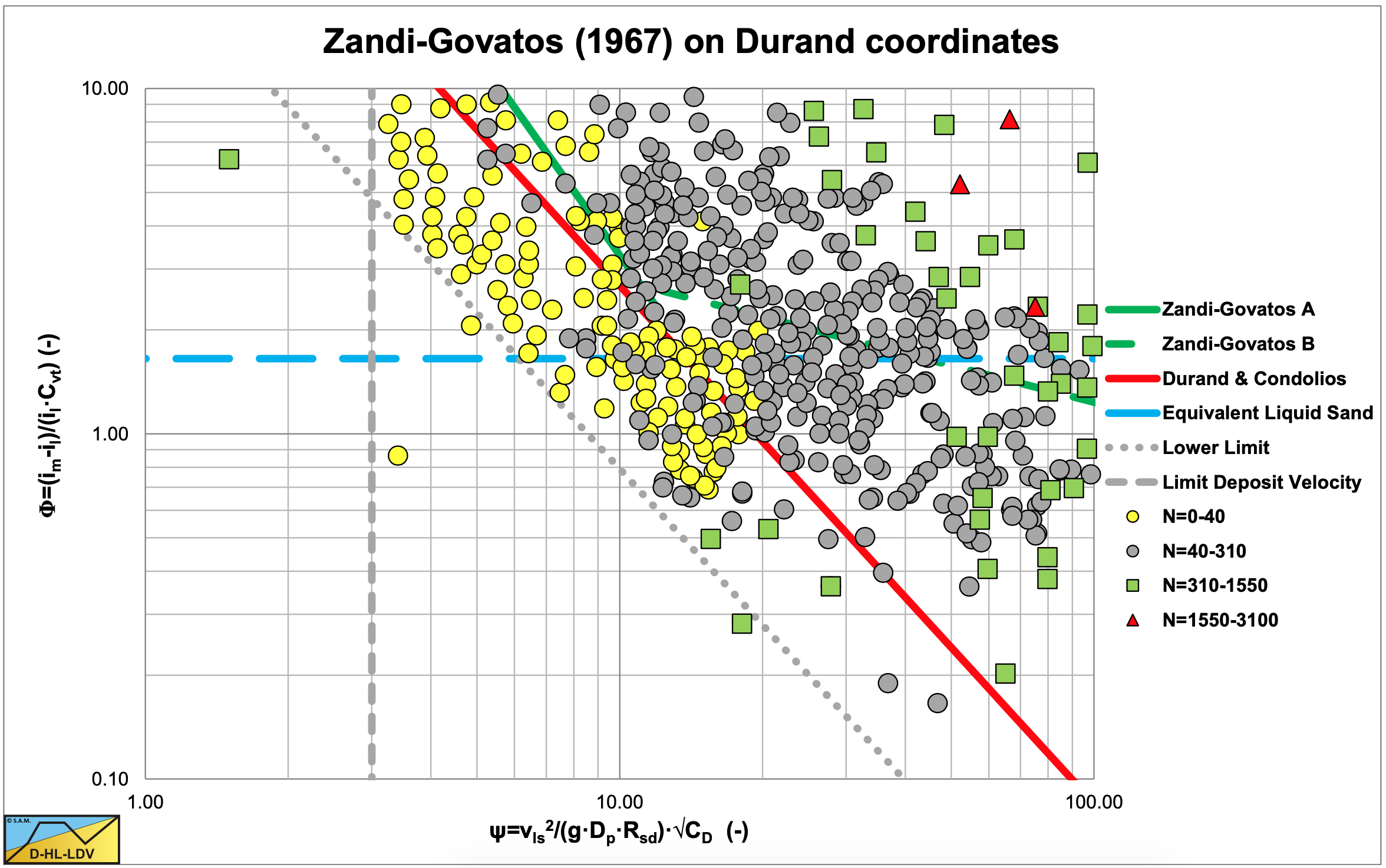
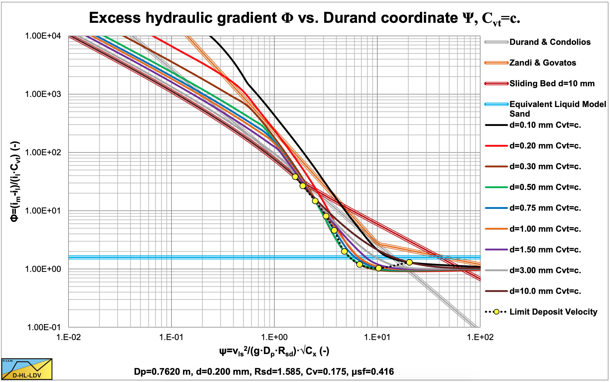
Figure 6.4-35 and Figure 6.4-36 show the results of the DHLLDV Framework for 2 pipe diameters in the same coordinate system as Figure 6.4-33 and Figure 6.4-34 for particles with diameters ranging from 0.1 mm to 10 mm and pipes with diameters of 0.1524 m (6 inch) and 0.762 m 30 inch. The results of the DHLLDV Framework match the data in Figure 6.4-33 very well. It should be noted that Figure 6.4-33 also contains data points with different relative submerged densities, while the DHLLDV Framework here only contains curves for sand and gravel. For the 0.1524 m diameter pipe the curves are around the Durand & Condolios curve, which could be expected. For the 0.762 diameter pipe the curves are in general below the Durand & Condolios curve. Between an abscissa of 1 and 10 the steepness of the curves matches the Zandi & Govatos curve. The behavior of the curves above an abscissa of about 10 explains for the steepness of the Zandi & Govatos curve in that area. At low values of the abscissa the steepness of the curves is less than at values above 1. This is caused by the fact that at low values there is a sliding bed, while at high values the transport is heterogeneous and at values above about 10 the flow is homogeneous.

Figure 6.4-35: The DHLLDV Framework for a 0.1524 m diameter pipe.

Figure 6.4-36: The DHLLDV Framework for a 0.762 m diameter pipe.

6.4.5 Issues Regarding the Durand & Condolios (1952) and Gibert (1960) Model

There are 8 issues to be discussed:

1. The drag coefficient of Durand & Condolios (1952) versus the real drag coefficient.
2. The drag coefficient as applied by Worster & Denny (1955),
3. The drag coefficient of Gibert (1960).
4. The relative submerged density as part of the equation.
5. The graph of Zandi & Govatos (1967).
6. The F_L value as published by many authors.
7. The Darcy Weisbach friction coefficient λ_l.
8. The solids effect term in the hydraulic gradient equation.

6.4.5.1 The Drag Coefficient of Durand & Condolios (1952) vs. the Real Drag Coefficient

It should be noted that Durand & Condolios (1952), Gibert (1960) and Worster & Denny (1955) use the particle Froude number in their equations and not the particle drag coefficient. The particle Froude number Fr_p is:

\[\ \mathrm{F r}_{\mathrm{p}}=\frac{\mathrm{v}_{\mathrm{t}}}{\sqrt{\mathrm{g} \cdot \mathrm{d}}}\]

The virtual drag coefficient as used by Durand & Condolios (1952), Gibert (1960) and Worster & Denny (1955), is:

\[\ \mathrm{C_{x}=\frac{g \cdot d}{v_{t}^{2}}=F r_{p}^{-2}}\]

The drag coefficient C_D as used in the equation for the terminal settling velocity is:

\[\ \begin{array}{left} \mathrm{v_{t}=\sqrt{\frac{4 \cdot g \cdot\left(\rho_{s}-\rho_{l}\right) \cdot d \cdot \Psi}{3 \cdot \rho_{l} \cdot C_{D}}}=\sqrt{\frac{4 \cdot g \cdot R_{s d} \cdot d \cdot \Psi}{3 \cdot C_{D}}} \Rightarrow C_{D}=\frac{4 \cdot R_{s d} \cdot \Psi}{3} \cdot \frac{g \cdot d}{v_{t}^{2}}} \\
{\mathrm{Fr}}_{\mathrm{p}}^{2}=\frac{\mathrm{v_{t}}^{2}}{\mathrm{g \cdot d}}=\frac{4}{3} \cdot \frac{\mathrm{R_{s d}} \cdot \Psi}{\mathrm{C_{D}}}\end{array}\]

So the relation between the drag coefficient C_D and the virtual drag coefficient according to Durand and Condolios (1952) C_x is:

\[\ \mathrm{C}_{\mathrm{D}}=\frac{\mathrm{4} \cdot \mathrm{R}_{\mathrm{s d}} \cdot \Psi}{\mathrm{3}} \cdot \mathrm{C}_{\mathrm{x}} \quad \text{ or }\quad \frac{\mathrm{1}}{\sqrt{\mathrm{C}_{\mathrm{x}}}}=\frac{\mathrm{v}_{\mathrm{t}}}{\sqrt{\mathrm{g} \cdot \mathrm{d}}}=\sqrt{\frac{4 \cdot \mathrm{R}_{\mathrm{s d}} \cdot \Psi}{\mathrm{3}}} \cdot \frac{\mathrm{1}}{\sqrt{\mathrm{C}_{\mathrm{D}}}}\]

For irregular shaped sand particles with a shape factor of ψ=0.5-0.7 and a relative submerged density of R_sd=1.65 this results in a drag coefficient almost equal to the Durand & Condolios (1952), Gibert (1960) and Worster coefficient. The term \(\ \mathrm{\frac{4 \cdot R_{s d} \cdot \Psi}{3}=2.2 \cdot \Psi}\) is almost unity for a shape factor of ψ=0.5 and since it is used by its square root, the error is just 5%. However for spheres with ψ=1.0 this factor is 2.2 which cannot be neglected. For solids with another relative submerged density however, there may be a much bigger difference. Zandi & Govatos (1967) and many others also use the Durand & Condolios (1952), Gibert (1960) and Worster coefficient, although they name it C_D. It is often not clear whether authors used the C_D value or just named it C_D, using the C_x value. Since the error depends on both the shape factor ψ and the relative submerged density R_sd, the original particle Froude number Fr_p should be used, because the relation of Durand & Condolios (1952), matching their experiments is based on this particle Froude number.

6.4.5.2 The Drag Coefficient as Applied by Worster & Denny (1955)

Worster & Denny (1955) applied a drag coefficient of 0.4 (source Bain & Bonnington (1970)) to make his data match the Durand & Condolios (1952) equation. Whether this is the C_D or the C_x is not important, because the numerical value is given. A value of 0.4 however is too small for irregular shaped coal. Spheres have a C_D value of 0.445 for turbulent settling. Sand particles may have a value of about 1. So the value used by Worster & Denny is questionable.

6.4.5.3 The Drag Coefficient of Gibert (1960)

Gibert (1960) published a table with numerical values for the virtual drag coefficient or particle Froude number. If one uses the values of Gibert (1960), the whole discussion about whether the C_D or the C_x value should be used can be omitted. Analyzing this table however, shows that a very good approximation of the table values can be achieved by using the particle Froude number to the power 20/9 instead of the power 1, assuming that the terminal settling velocity vt is determined correctly for the solids considered (Stokes, Budryck, Rittinger or Zanke).

\[\ \sqrt{\mathrm{C}_{\mathrm{x}, \mathrm{G i b e r t}}}=\sqrt{\mathrm{C}_{\mathrm{x}}}^ \mathrm{2 0 / 9}\]

Together with the correction of Gibert (1960), regarding the constant of 85/180, the equation now becomes:

\[\ \Delta \mathrm{p}_{\mathrm{m}}=\Delta \mathrm{p_{l}} \cdot\left(1+\Phi \cdot \mathrm{C}_{\mathrm{vt}}\right) \quad\text{ with: }\quad \Phi=85 \cdot\left(\frac{\mathrm{v}_{\mathrm{ls}}^{2} \cdot \mathrm{C}_{\mathrm{x}}^{10 / 9}}{\mathrm{g} \cdot \mathrm{D}_{\mathrm{p}} \cdot \mathrm{R}_{\mathrm{sd}}}\right)^{-3 / 2}\]

6.4.5.4 The Relative Submerged Density as Part of the Equation

In a number of books and publications the relative submerged density R_sd is added to both the flow Froude number Fr_fl and the particle Froude number Fr_p. This, to enable the use of the equations for different types of solids. Gibert (1960) clearly states that the relative submerged density should only be added to the flow Froude number Fr_fl and not to the particle Froude number Fr_p, since it is already part of the terminal settling velocity v_t. Equations (6.4-41) and (6.4-45) are thus the final equations of the Durand & Condolios (1952) and Gibert (1960) model.

6.4.5.5 The Graph of Zandi & Govatos (1967)

The famous graph of Zandi & Govatos (1967) showing many data points on Φ-Ψ coordinates, is often incorrect. The lines of the Durand & Condolios (1952) equation and the line of pseudo homogeneous transport by Zandi & Govatos (1967) are reproduced incorrectly. Only the line of heterogeneous transport by Zandi & Govatos (1967) is correct. Probably this happened by copy paste, but it shows a wrong relation between the data points and the equations. Only in the book of Raudviki (1990) a correct graph is found. Raudviki also gives a good view on the location of the data points and the location of the equivalent liquid model for sand.

6.4.5.6 The FL Value as Published by Many Authors

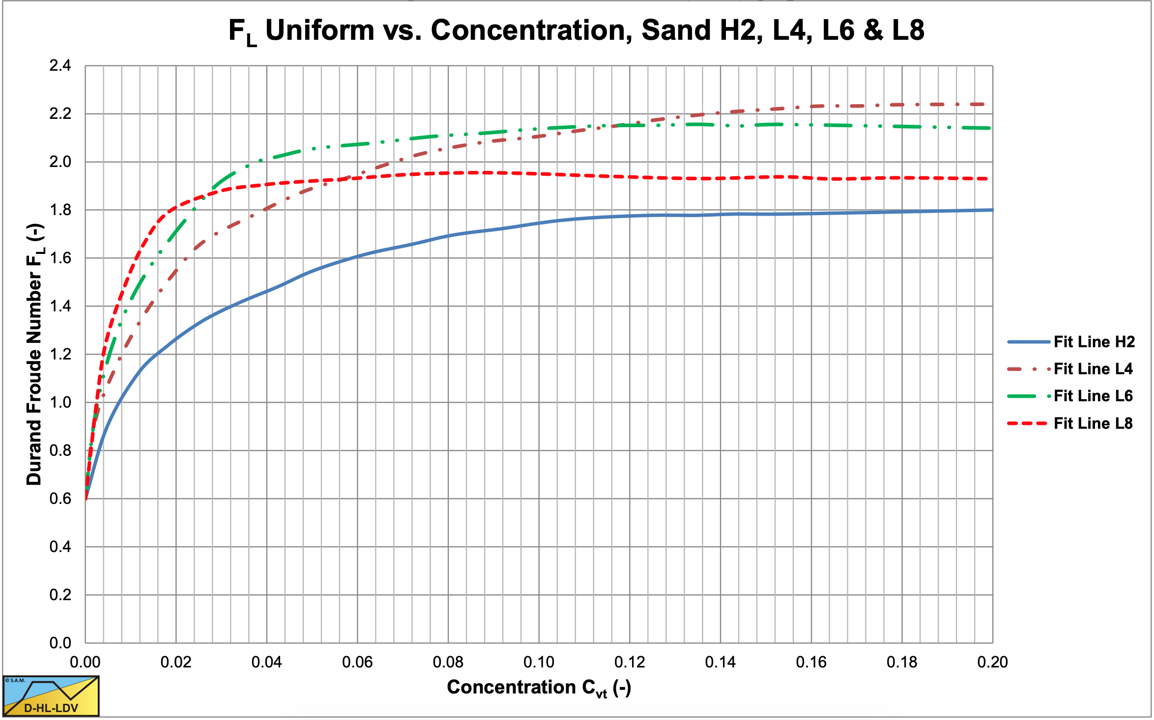
The issue of the Limit Deposit Velocity Froude number F_L is of great importance. In their original publication, Durand & Condolios (1952) published 4 graphs showing the F_L value as a function of the volumetric transport concentration C_vt for the sands H2, L4, L6 and L8 (4 different particle diameters), these graphs are summarized in Figure 6.4-37. The Limit Deposit Velocity Froude number is defined as:

\[\ \mathrm{F}_{\mathrm{L}}=\mathrm{F r}_{\mathrm{l d v}}=\frac{\mathrm{v}_{\mathrm{l s}, \mathrm{ld} \mathrm{v}}}{\sqrt{\mathrm{g} \cdot \mathrm{D}_{\mathrm{p}}}}\]

Based on Figure 6.4-37 the relation between F_L and the particle diameter d can be derived at different concentrations, which is shown in Figure 6.4-38.
With some curve fitting and extrapolation the graph as published by Durand & Condolios (1952) was constructed. The graphs as shown here are directly constructed from the original data points, without curve fitting and/or extrapolation. The graph as published has an asymptotic value for large particle diameters of about 1.9. Figure 6.4-22 shows a reconstruction of the original Durand & Condolios (1952) graph.

Figure 6.4-37: The trend lines of the F_L value as a function of the concentration.

Figure 6.4-38: The trend lines of the F_L value as a function of the particle diameter.

Durand (1953) published his findings in the English language, while the original paper was in the French language. He modified the F_L coefficient, by including the relative submerged density and a factor 2, but he divided the vertical axis only by \(\ \sqrt{2}\), resulting in an asymptotic value of 1.34. Since (probably) most authors of books and publications read the English paper from 1953, this graph was copied and can be found in almost every text book about slurry transport. The vertical axis should have been divided by \(\ \sqrt{2 \cdot \mathrm{R}_{\mathrm{sd}}}\) resulting in an asymptotic value of about 1.05, a difference of about 28% or the square root of 1.65.

Now which one of the graphs is correct? Based on LDV’s reported by Durand & Condolios (1952) between 2.9 and 3.2 m/s for a 0.1524 diameter pipe, F_L values between 1.34 and 1.48 should be expected. So the conclusion is that the graph of Durand (1953) is the correct graph and in the graph of Durand & Condolios (1952) the data were already divided by the square root of 1.65. The correct graph is shown in Figure 6.4-24.

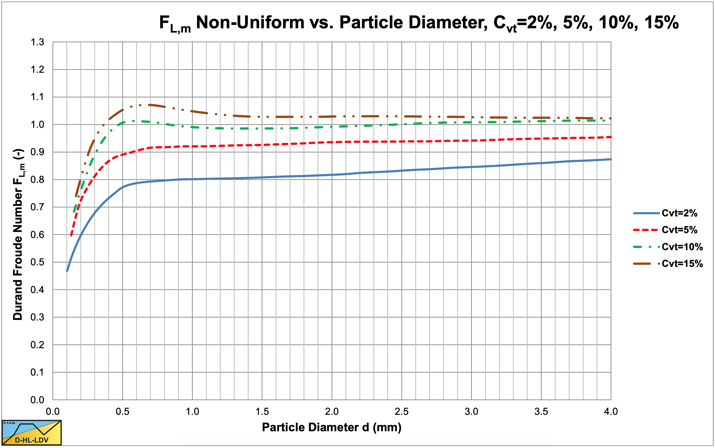
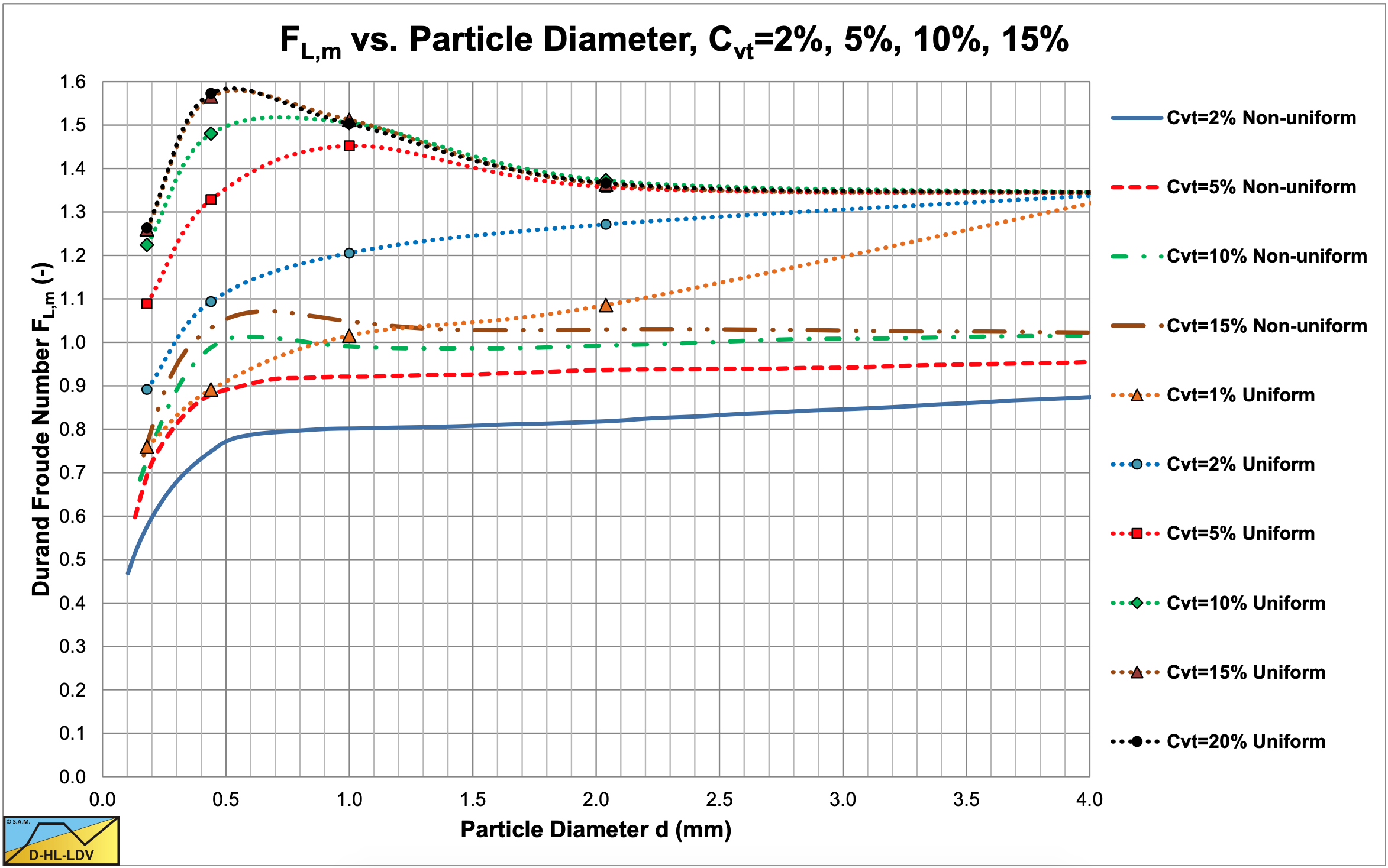
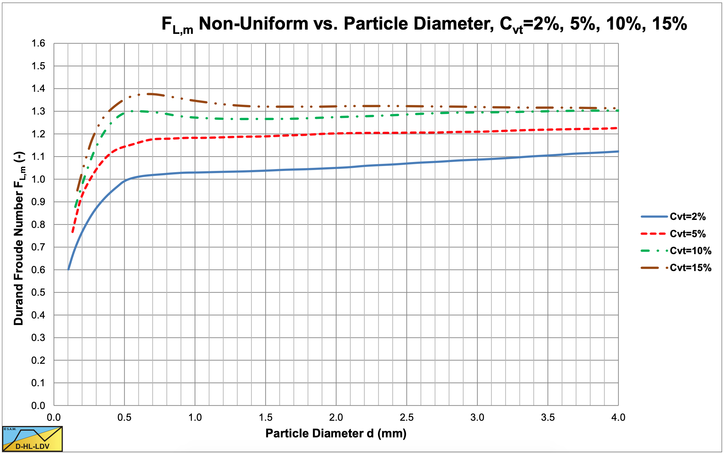
Later Durand & Condolios (1956) published a graph for non-uniform particle size distributions, where the original Durand & Condolios (1952) graph is considered to be for uniform particle size distributions. Figure 6.4-39 shows the graph of Condolios & Chapus. Figure 6.4-40 gives a comparison of the F_L value for uniform and non-uniform particle size distributions. The trends of uniform and non-uniform particle size distributions are the same, but non- uniform particle size distributions have, in general a much smaller F_L value, at the same d₅₀. This results in much smaller Limit Deposit Velocities. This does not seem to be reasonable. There is no physical explanation for example, why graded coarse particles would have a much lower LDV if they are mixed. The same limiting F_L value of about 1.34 would be expected if all individual particles have this value. An error of the square root of the relative submerged density could be the explanation. So the graph is corrected for the relative submerged density, while it shouldn’t. Figure 6.4-41 shows the graph for non-uniform distributed particles corrected for the relative submerged density, while Figure 6.4-42 shows the comparison uniform versus non-uniform distributions. For coarse particles they give similar F_L values for concentrations of 15%-20%. For medium sized particles non- uniform distributed particles give smaller values, but still there is not too much difference. It is assumed in this book that Figure 6.4-42 is the correct graph.

Apparently the original data were determined with:

\[\ \mathrm{F}_{\mathrm{L}, \mathrm{o r i g i n a l}}=\frac{\mathrm{v}_{\mathrm{l s}, \mathrm{d} \mathrm{v}}}{\sqrt{\mathrm{g} \cdot \mathrm{D}_{\mathrm{p}} \cdot \mathrm{R}_{\mathrm{s d}}}}\]

Instead of:

\[\ \mathrm{F}_{\mathrm{L}, \mathrm{o r i g i n a l}}=\frac{\mathrm{v}_{\mathrm{l s}, \mathrm{l d v}}}{\sqrt{\mathrm{g} \cdot \mathrm{D}_{\mathrm{p}}}}\]

The final formulation is now:

\[\ \mathrm{F}_{\mathrm{L}}=\mathrm{F}_{\mathrm{L}, \mathrm{o r i g i n a l}} \cdot \frac{\mathrm{1}}{\sqrt{2}}=\frac{\mathrm{v}_{\mathrm{l s}, \mathrm{d v}}}{\sqrt{\mathrm{2 \cdot g} \cdot \mathrm{D}_{\mathrm{p}} \cdot \mathrm{R}_{\mathrm{s d}}}}\]

Instead of:

\[\ \mathrm{F}_{\mathrm{L}}=\mathrm{F}_{\mathrm{L}, \mathrm{o r i g i n a l}} \cdot \frac{\mathrm{1}}{\sqrt{\mathrm{2 \cdot R}_{\mathrm{s d}}}}=\frac{\mathrm{v}_{\mathrm{l s}, \mathrm{l d v}}}{\sqrt{\mathrm{2 \cdot g} \cdot \mathrm{D}_{\mathrm{p}} \cdot \mathrm{R}_{\mathrm{s d}}}}\]

Figure 6.4-39: The trend lines of the F_L value as a function of the particle diameter for non-uniform distributions.

Figure 6.4-40: Comparing uniform and non-uniform distributions.

Figure 6.4-41: The trend lines of the F_L value as a function of the particle diameter for non-uniform distributions, modified.

Figure 6.4-42: Comparing uniform and non-uniform distributions, modified.

6.4.5.7 The Darcy-Weisbach Friction Coefficient λ_l

Many researchers use the following equation for the contribution of the solids to the pressure losses:

\[\ \mathrm{i}_{\mathrm{m}}=\mathrm{i}_{\mathrm{l}} \cdot\left(\mathrm{1}+\mathrm{\Phi} \cdot \mathrm{C}_{\mathrm{v t}}\right)\]

Some other researchers disconnected the solids effect from the hydraulic gradient i_fl, implying that the solids effect is independent from the hydraulic gradient, according to:

\[\ \mathrm{i}_{\mathrm{m}}=\mathrm{i}_{\mathrm{l}}+\mathrm{\Phi} \cdot \mathrm{C}_{\mathrm{v} \mathrm{t}}\]

Of course the formulation of Φ is different in both equations. Since the hydraulic gradient i_fl depends strongly on the value of the friction coefficient λ_l, the formulation of equation (6.4-51) also depends strongly on the friction coefficient λ_l, while the formulation of equation (6.4-52) does not.

Since the friction coefficient λ_l may vary from about 0.01 for large smooth pipes (D_p=1 m) to about 0.04 for small smooth pipes (D_p=0.0254 m), a difference of a factor 4 may occur between both equations when extrapolating from a very small pipe in a laboratory to a large pipe in reality. Since most experiments are carried out in small to medium pipe diameters (D_p=0.0254 m to D_p=0.254 m), this should be taken into consideration. It is thus important to know whether the solids effect depends on the friction coefficient λ_l or not. If it does a formulation like equation (6.4-51) should be used, if it does not a formulation like equation (6.4-52) should be used. The Durand & Condolios (1952) equation in this form will look like:

\[\ \begin{array}{left}\mathrm{i}_{\mathrm{m}}&=\mathrm{i}_{\mathrm{l}} \cdot\left(\mathrm{1}+\mathrm{8 5} \cdot\left(\frac{\mathrm{v}_{\mathrm{l} \mathrm{s}}^{2} \cdot \mathrm{C}_{\mathrm{x}}}{\mathrm{g} \cdot \mathrm{D}_{\mathrm{p}} \cdot \mathrm{R}_{\mathrm{s d}}}\right)^{-\mathrm{3} / \mathrm{2}} \cdot \mathrm{C}_{\mathrm{v t}}\right)\\
&=\mathrm{i}_{\mathrm{l}}+\mathrm{8 5} \cdot \frac{\lambda_{1} \cdot \mathrm{R}_{\mathrm{s d}}}{\mathrm{2}} \cdot\left(\frac{\mathrm{v}_{\mathrm{l} \mathrm{s}}^{2}}{\mathrm{g} \cdot \mathrm{D}_{\mathrm{p}} \cdot \mathrm{R}_{\mathrm{s d}}}\right)^{2 / 2} \cdot\left(\frac{\mathrm{g} \cdot \mathrm{D}_{\mathrm{p}} \cdot \mathrm{R}_{\mathrm{s} \mathrm{d}}}{\mathrm{v}_{\mathrm{l} \mathrm{s}}^{2}}\right)^{3 / 2} \cdot\left(\frac{\mathrm{1}}{\mathrm{C}_{\mathrm{x}}}\right)^{3 / 2} \cdot \mathrm{C}_{\mathrm{v} \mathrm{t}}\end{array}\]

With R_sd=1.65 for sands and gravels this gives:

\[\ \mathrm{i}_{\mathrm{m}}=\mathrm{i}_{\mathrm{l}}+\mathrm{7 0} \cdot \lambda_{\mathrm{l}} \cdot\left(\frac{\mathrm{g} \cdot \mathrm{D}_{\mathrm{p}} \cdot \mathrm{R}_{\mathrm{s d}}}{\mathrm{v}_{\mathrm{l s}}^{\mathrm{2}}}\right)^{1 / 2} \cdot\left(\frac{\mathrm{1}}{\mathrm{C}_{\mathrm{x}}}\right)^{3 / 2} \cdot \mathrm{C}_{\mathrm{v t}}\]

This last equation will give the same results as the original equation for sands and gravels. For pipe diameters from D_p=0.0254 m to D_p=1 m, the friction factor λ_l decreases about the same factor as the increase of the square root of the pipe diameter D_p, meaning that the excess pressure losses are almost independent of the pipe diameter D_p.

6.4.5.8 The Solids Effect Term in the Hydraulic Gradient Equation

In both equations (6.4-51) and (6.4-52), the solids effect is incorporated as one term Φ. This term often consists of a one term equation, often based on Froude numbers. Now the question is whether the solids effect can be described physically by a one term equation. It is very well possible that the solids effect depends on a number of different physical phenomena, each with its own term in the equation. Using just one term may force the curve fit equations, as used by most researchers, into a low correlation equation, just because a one term equation does not describe the processes involved accurately. Using Froude numbers forces the fit equation in a fixed ratio between a number of parameters involved. The flow Froude number forces a fixed ratio between the line speed and the pipe diameter, while the particle Froude number forces a fixed ratio between the terminal settling velocity and the particle diameter. Using an equation for the solids effect with more than one term, without fixing certain ratio’s, would probably give a better correlation with the experimental data.