
6.7: Graf et al. (1970) and Robinson (1971)
- Page ID
- 30850

\( \newcommand{\vecs}[1]{\overset { \scriptstyle \rightharpoonup} {\mathbf{#1}} } \)
\( \newcommand{\vecd}[1]{\overset{-\!-\!\rightharpoonup}{\vphantom{a}\smash {#1}}} \)
\( \newcommand{\id}{\mathrm{id}}\) \( \newcommand{\Span}{\mathrm{span}}\)
( \newcommand{\kernel}{\mathrm{null}\,}\) \( \newcommand{\range}{\mathrm{range}\,}\)
\( \newcommand{\RealPart}{\mathrm{Re}}\) \( \newcommand{\ImaginaryPart}{\mathrm{Im}}\)
\( \newcommand{\Argument}{\mathrm{Arg}}\) \( \newcommand{\norm}[1]{\| #1 \|}\)
\( \newcommand{\inner}[2]{\langle #1, #2 \rangle}\)
\( \newcommand{\Span}{\mathrm{span}}\)
\( \newcommand{\id}{\mathrm{id}}\)
\( \newcommand{\Span}{\mathrm{span}}\)
\( \newcommand{\kernel}{\mathrm{null}\,}\)
\( \newcommand{\range}{\mathrm{range}\,}\)
\( \newcommand{\RealPart}{\mathrm{Re}}\)
\( \newcommand{\ImaginaryPart}{\mathrm{Im}}\)
\( \newcommand{\Argument}{\mathrm{Arg}}\)
\( \newcommand{\norm}[1]{\| #1 \|}\)
\( \newcommand{\inner}[2]{\langle #1, #2 \rangle}\)
\( \newcommand{\Span}{\mathrm{span}}\) \( \newcommand{\AA}{\unicode[.8,0]{x212B}}\)
\( \newcommand{\vectorA}[1]{\vec{#1}} % arrow\)
\( \newcommand{\vectorAt}[1]{\vec{\text{#1}}} % arrow\)
\( \newcommand{\vectorB}[1]{\overset { \scriptstyle \rightharpoonup} {\mathbf{#1}} } \)
\( \newcommand{\vectorC}[1]{\textbf{#1}} \)
\( \newcommand{\vectorD}[1]{\overrightarrow{#1}} \)
\( \newcommand{\vectorDt}[1]{\overrightarrow{\text{#1}}} \)
\( \newcommand{\vectE}[1]{\overset{-\!-\!\rightharpoonup}{\vphantom{a}\smash{\mathbf {#1}}}} \)
\( \newcommand{\vecs}[1]{\overset { \scriptstyle \rightharpoonup} {\mathbf{#1}} } \)
\( \newcommand{\vecd}[1]{\overset{-\!-\!\rightharpoonup}{\vphantom{a}\smash {#1}}} \)
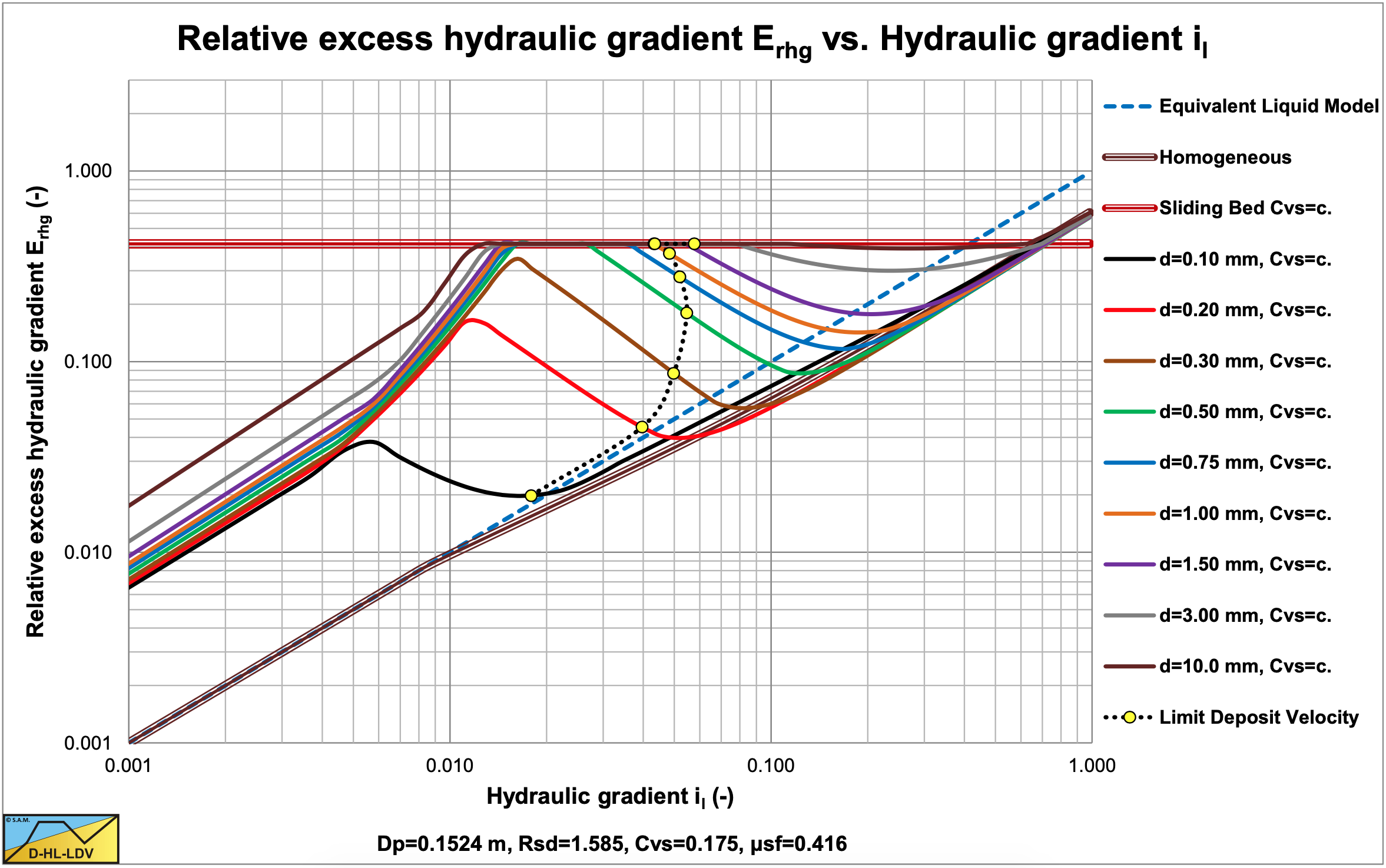
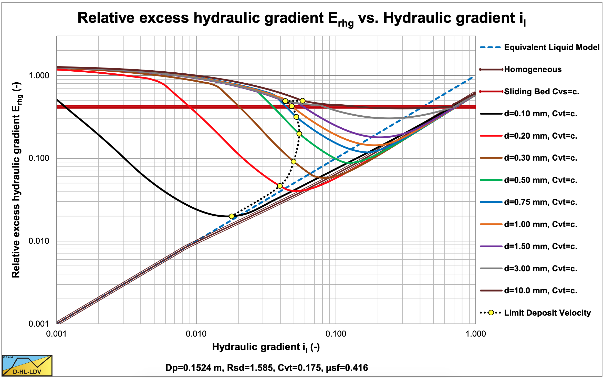
\(\newcommand{\avec}{\mathbf a}\) \(\newcommand{\bvec}{\mathbf b}\) \(\newcommand{\cvec}{\mathbf c}\) \(\newcommand{\dvec}{\mathbf d}\) \(\newcommand{\dtil}{\widetilde{\mathbf d}}\) \(\newcommand{\evec}{\mathbf e}\) \(\newcommand{\fvec}{\mathbf f}\) \(\newcommand{\nvec}{\mathbf n}\) \(\newcommand{\pvec}{\mathbf p}\) \(\newcommand{\qvec}{\mathbf q}\) \(\newcommand{\svec}{\mathbf s}\) \(\newcommand{\tvec}{\mathbf t}\) \(\newcommand{\uvec}{\mathbf u}\) \(\newcommand{\vvec}{\mathbf v}\) \(\newcommand{\wvec}{\mathbf w}\) \(\newcommand{\xvec}{\mathbf x}\) \(\newcommand{\yvec}{\mathbf y}\) \(\newcommand{\zvec}{\mathbf z}\) \(\newcommand{\rvec}{\mathbf r}\) \(\newcommand{\mvec}{\mathbf m}\) \(\newcommand{\zerovec}{\mathbf 0}\) \(\newcommand{\onevec}{\mathbf 1}\) \(\newcommand{\real}{\mathbb R}\) \(\newcommand{\twovec}[2]{\left[\begin{array}{r}#1 \\ #2 \end{array}\right]}\) \(\newcommand{\ctwovec}[2]{\left[\begin{array}{c}#1 \\ #2 \end{array}\right]}\) \(\newcommand{\threevec}[3]{\left[\begin{array}{r}#1 \\ #2 \\ #3 \end{array}\right]}\) \(\newcommand{\cthreevec}[3]{\left[\begin{array}{c}#1 \\ #2 \\ #3 \end{array}\right]}\) \(\newcommand{\fourvec}[4]{\left[\begin{array}{r}#1 \\ #2 \\ #3 \\ #4 \end{array}\right]}\) \(\newcommand{\cfourvec}[4]{\left[\begin{array}{c}#1 \\ #2 \\ #3 \\ #4 \end{array}\right]}\) \(\newcommand{\fivevec}[5]{\left[\begin{array}{r}#1 \\ #2 \\ #3 \\ #4 \\ #5 \\ \end{array}\right]}\) \(\newcommand{\cfivevec}[5]{\left[\begin{array}{c}#1 \\ #2 \\ #3 \\ #4 \\ #5 \\ \end{array}\right]}\) \(\newcommand{\mattwo}[4]{\left[\begin{array}{rr}#1 \amp #2 \\ #3 \amp #4 \\ \end{array}\right]}\) \(\newcommand{\laspan}[1]{\text{Span}\{#1\}}\) \(\newcommand{\bcal}{\cal B}\) \(\newcommand{\ccal}{\cal C}\) \(\newcommand{\scal}{\cal S}\) \(\newcommand{\wcal}{\cal W}\) \(\newcommand{\ecal}{\cal E}\) \(\newcommand{\coords}[2]{\left\{#1\right\}_{#2}}\) \(\newcommand{\gray}[1]{\color{gray}{#1}}\) \(\newcommand{\lgray}[1]{\color{lightgray}{#1}}\) \(\newcommand{\rank}{\operatorname{rank}}\) \(\newcommand{\row}{\text{Row}}\) \(\newcommand{\col}{\text{Col}}\) \(\renewcommand{\row}{\text{Row}}\) \(\newcommand{\nul}{\text{Nul}}\) \(\newcommand{\var}{\text{Var}}\) \(\newcommand{\corr}{\text{corr}}\) \(\newcommand{\len}[1]{\left|#1\right|}\) \(\newcommand{\bbar}{\overline{\bvec}}\) \(\newcommand{\bhat}{\widehat{\bvec}}\) \(\newcommand{\bperp}{\bvec^\perp}\) \(\newcommand{\xhat}{\widehat{\xvec}}\) \(\newcommand{\vhat}{\widehat{\vvec}}\) \(\newcommand{\uhat}{\widehat{\uvec}}\) \(\newcommand{\what}{\widehat{\wvec}}\) \(\newcommand{\Sighat}{\widehat{\Sigma}}\) \(\newcommand{\lt}{<}\) \(\newcommand{\gt}{>}\) \(\newcommand{\amp}{&}\) \(\definecolor{fillinmathshade}{gray}{0.9}\)Graf et al. (1970), Robinson (1971) and Robinson & Graf (1972) conducted experiments on critical deposit velocities for low concentration (Cvs<5%) solid liquid mixtures. The critical deposit velocity is defined here as the velocity at which particles begin to settle from the carrying medium and form a stationary (non-moving) deposit along the invert of the pipe. Since many definitions exist, it is important to keep this definition in mind when interpreting the data. Others defined the critical deposit velocity as the velocity at which particles begin to settle from the carrying medium and form a stationary or sliding deposit along the invert of the pipe, which could give different results, a higher critical deposit velocity. The latter is defined in this book as the LDV, the Graf & Robinson definition as the LSDV. Others use the definition of the minimum hydraulic gradient velocity, referred to in this book as the MHGV. It should be mentioned here that for very fine particles a sliding bed will not occur and the LDV and LSDV are the same. The study was concerned with settling mixtures, which exhibit Newtonian flow characteristics and was analyzed as a two phase flow phenomenon. 4 flow regimes are distinguished, the deposit regime, a separation regime between deposit and no deposit, heterogeneous flow with and without saltation and the pseudo homogeneous regime. The points of division between different flow regimes is somewhat arbitrary. Figure 6.10-2 and Figure 6.10-3 show the different flow regimes for constant spatial and constant delivered volumetric concentration. The simulations are carried out with the DHLLDV Framework and are similar to the graphs shown by Graf & Robinson.
\[\ \mathrm{F}_{\mathrm{L}}=\frac{\mathrm{v}_{\mathrm{l s}, \mathrm{l d v}}}{\sqrt{\mathrm{2 \cdot g} \cdot \mathrm{D}_{\mathrm{p}} \cdot \mathrm{R}_{\mathrm{s d}}}}\]
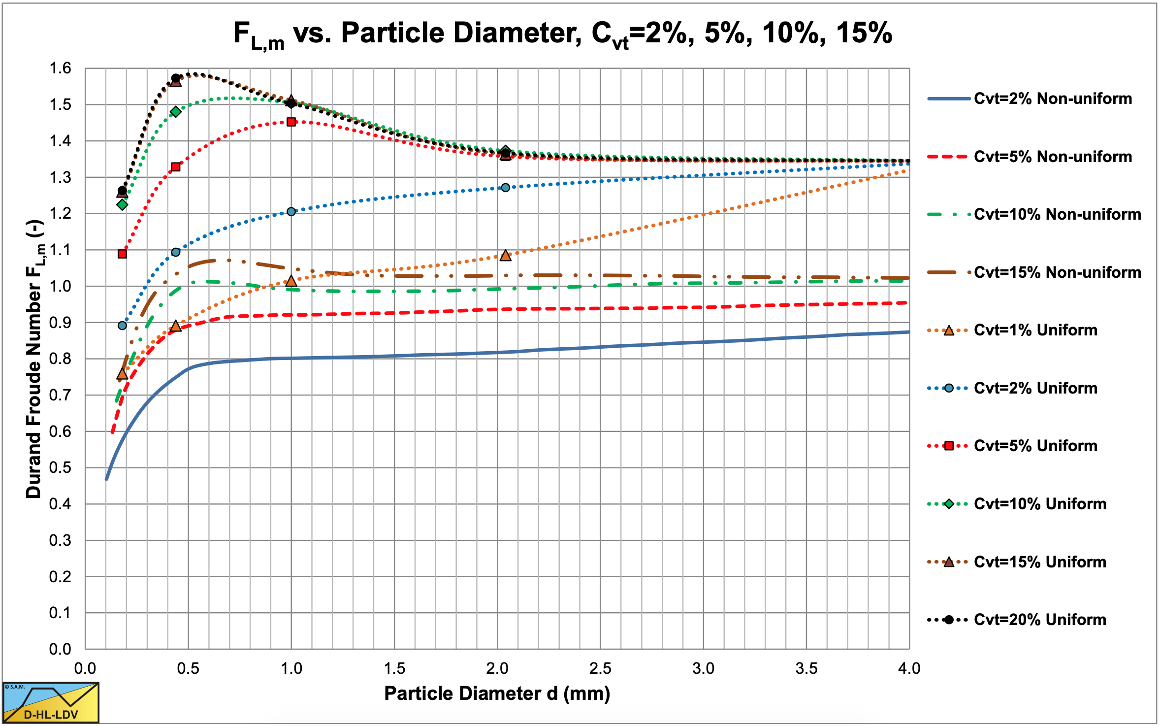
Graf & Robinson used the Froude number FL, as defined by Durand & Condolios (1952) as a reference. They noted that the curves for uniform sands, as shown in Figure 6.10-1, are too high, while the curves for non-uniform sands seem reasonable. The reason for this is discussed in the chapter about Durand& Condolios, the curves for uniform sands are a factor 1.285 too high. Graf & Robinson then reconstructed the graph based on the Gibert (1960) data, resulting in a graph very similar to the graph of the non-uniform sands, only with slightly higher curves with concentrations up to 10%. Sinclair (1962) found an upper limit of 1.24 for the FL value, using:
\[\ \mathrm{F_{L, \max }}=\frac{\mathrm{v_{\mathrm{ls}, \mathrm{ldv}, \max }}}{\sqrt{2 \cdot \mathrm{g} \cdot \mathrm{D}_{\mathrm{p}} \cdot \mathrm{R}_{\mathrm{sd}}}}=1.3 \cdot \sqrt{\mathrm{R}_{\mathrm{sd}}^{-0.2}}\]
The upper limit of Durand & Condolios (1952) is about 1.05, while the Gibert (1960) data result in an upper limit of about 1.27. The pipe diameters in all experiments considered here, resulting in the maximum FL value, are up to 0.1524 m (6 inch).
The experiments of Graf & Robinson were carried out with two pipe diameters, a Dp=0.1016 m diameter pipe (4 inch) and a Dp=0.1524 m diameter pipe (6 inch). Two sands were used, a sand with d=0.45 mm and a sand with d=0.88 mm. Also tests with plastic pellets with d=3.63 mm were carried out. The experiments were carried out with constant spatial volumetric concentration, although a lot of scatter was observed. The concentration measured was the delivered volumetric concentration. They also used slightly inclined pipes with positive (θ=1.5o and tan(θ)=0.027) and negative (θ=-3.5o and tan(θ)=-0.06) angles, resulting in a modified FL number:
\[\ \mathrm{F}_{\mathrm{L}}=\frac{\mathrm{v}_{\mathrm{l} \mathrm{s}, \mathrm{ld v}}}{\sqrt{\mathrm{2 \cdot g} \cdot \mathrm{D}_{\mathrm{p}} \cdot \mathrm{R}_{\mathrm{s d}}}} \cdot(\mathrm{1}-\tan (\theta))\]
Assuming the concentration was the only important parameter, the following fit function was found:
\[\ \mathrm{F_{L}}=\frac{\mathrm{v_{l s, ld v}}}{\sqrt{\mathrm{2 \cdot g \cdot D_{p} \cdot R_{s d}}}} \cdot(1-\tan (\theta))=0.901 \cdot \mathrm{C_{v}^{0.106}}\]
Including the particle diameter in the correlation, the following equation was found:
\[\ \mathrm{F_{L}}=\frac{\mathrm{v_{l s, l d v}}}{\sqrt{\mathrm{2 \cdot g \cdot D_{p} \cdot R_{s d}}}} \cdot(1-\tan (\theta))=0.928 \cdot \mathrm{C_{v}^{0.105} \cdot d^{0.058}}\]
It should be mentioned that the concentration was limited to 7% and was most probably based on the spatial volumetric concentration. Meaning a fixed amount of solids in the test loop. Figure 6.10-4 shows the Durand Froude numbers as a function of the concentration, including the above fit line. At a concentration of 15-20%, which is often considered to give the highest LDV, the estimated FL value is 1.24. The data points of the plastic pellets seem to give higher Durand Froude numbers. The plastic pellets have a relative submerged density Rsd=0.34, which is low. Apparently the Durand Froude number increases with decreasing relative submerged density.
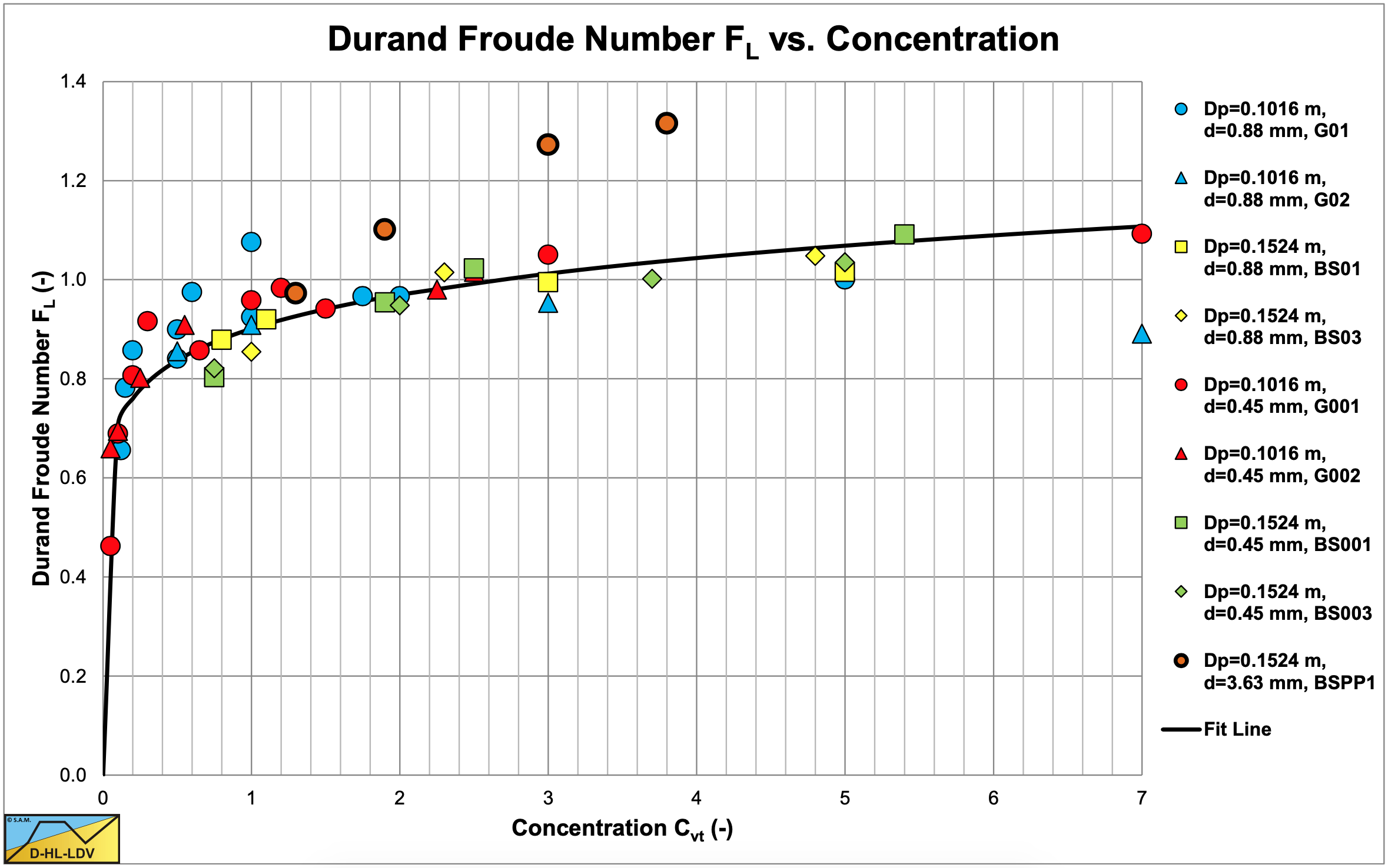
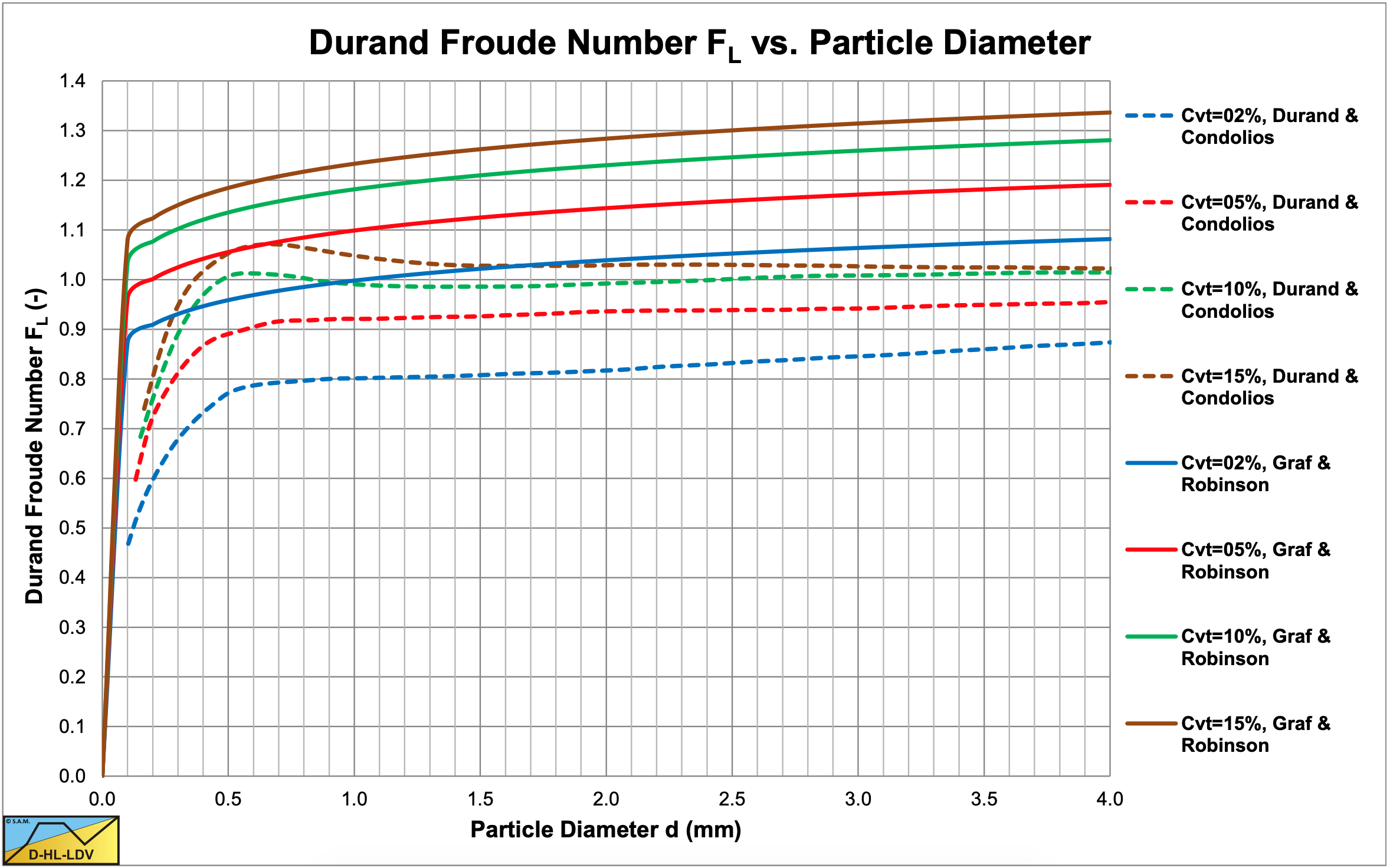
Figure 6.10-5 shows a comparison of the above equation (6.10-5) with the Durand & Condolios (1956) graph for non-uniform sands. It is clear that the above equation (6.10-5) gives considerable higher values for the Durand Froude number FL.
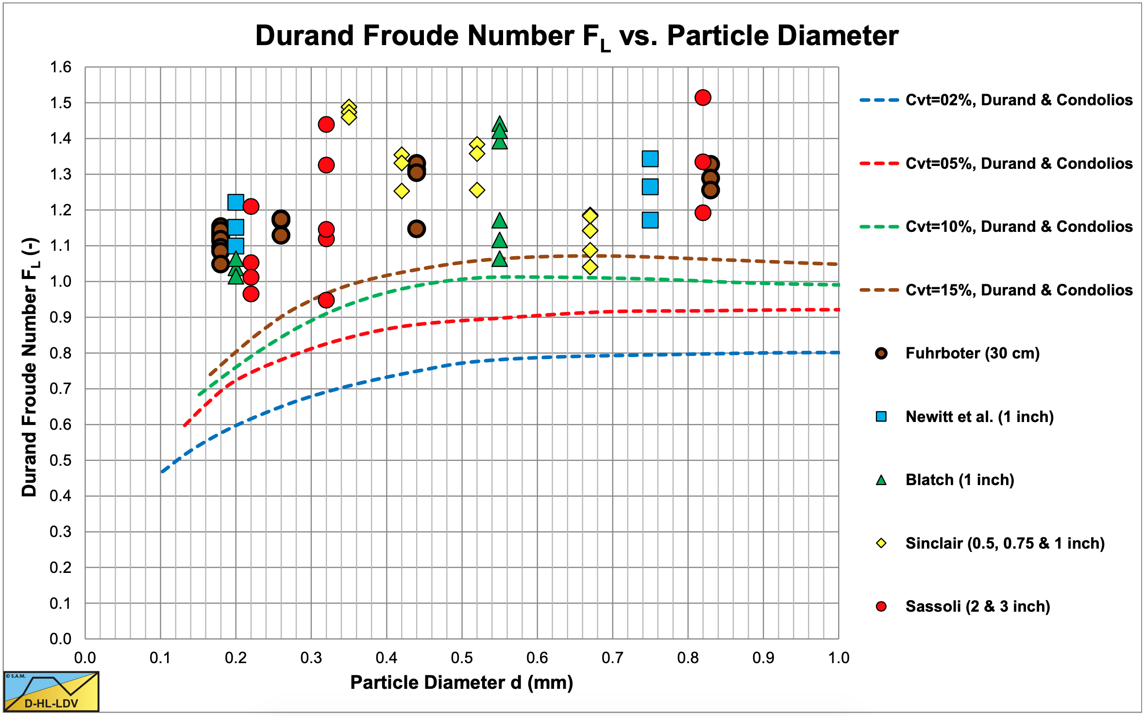
Graf et al. (1970) also show Durand FL values of some other researchers as is shown in Figure 6.10-6. The values are much larger than the ones predicted by the Durand & Condolios (1956). It is also noteworthy to mention that apparently the smaller pipe diameters result in larger FL values. The Fuhrboter (1961) values in a 30 cm (12 inch) pipe are smaller than the other values in much smaller pipes. The maximum values in each column are for concentrations between 15% and 20%. So it looks like the FL value decreases slightly with increasing pipe diameter.