
6.11: Kazanskij (1978) and (1980)
- Page ID
- 31044

\( \newcommand{\vecs}[1]{\overset { \scriptstyle \rightharpoonup} {\mathbf{#1}} } \)
\( \newcommand{\vecd}[1]{\overset{-\!-\!\rightharpoonup}{\vphantom{a}\smash {#1}}} \)
\( \newcommand{\id}{\mathrm{id}}\) \( \newcommand{\Span}{\mathrm{span}}\)
( \newcommand{\kernel}{\mathrm{null}\,}\) \( \newcommand{\range}{\mathrm{range}\,}\)
\( \newcommand{\RealPart}{\mathrm{Re}}\) \( \newcommand{\ImaginaryPart}{\mathrm{Im}}\)
\( \newcommand{\Argument}{\mathrm{Arg}}\) \( \newcommand{\norm}[1]{\| #1 \|}\)
\( \newcommand{\inner}[2]{\langle #1, #2 \rangle}\)
\( \newcommand{\Span}{\mathrm{span}}\)
\( \newcommand{\id}{\mathrm{id}}\)
\( \newcommand{\Span}{\mathrm{span}}\)
\( \newcommand{\kernel}{\mathrm{null}\,}\)
\( \newcommand{\range}{\mathrm{range}\,}\)
\( \newcommand{\RealPart}{\mathrm{Re}}\)
\( \newcommand{\ImaginaryPart}{\mathrm{Im}}\)
\( \newcommand{\Argument}{\mathrm{Arg}}\)
\( \newcommand{\norm}[1]{\| #1 \|}\)
\( \newcommand{\inner}[2]{\langle #1, #2 \rangle}\)
\( \newcommand{\Span}{\mathrm{span}}\) \( \newcommand{\AA}{\unicode[.8,0]{x212B}}\)
\( \newcommand{\vectorA}[1]{\vec{#1}} % arrow\)
\( \newcommand{\vectorAt}[1]{\vec{\text{#1}}} % arrow\)
\( \newcommand{\vectorB}[1]{\overset { \scriptstyle \rightharpoonup} {\mathbf{#1}} } \)
\( \newcommand{\vectorC}[1]{\textbf{#1}} \)
\( \newcommand{\vectorD}[1]{\overrightarrow{#1}} \)
\( \newcommand{\vectorDt}[1]{\overrightarrow{\text{#1}}} \)
\( \newcommand{\vectE}[1]{\overset{-\!-\!\rightharpoonup}{\vphantom{a}\smash{\mathbf {#1}}}} \)
\( \newcommand{\vecs}[1]{\overset { \scriptstyle \rightharpoonup} {\mathbf{#1}} } \)
\( \newcommand{\vecd}[1]{\overset{-\!-\!\rightharpoonup}{\vphantom{a}\smash {#1}}} \)
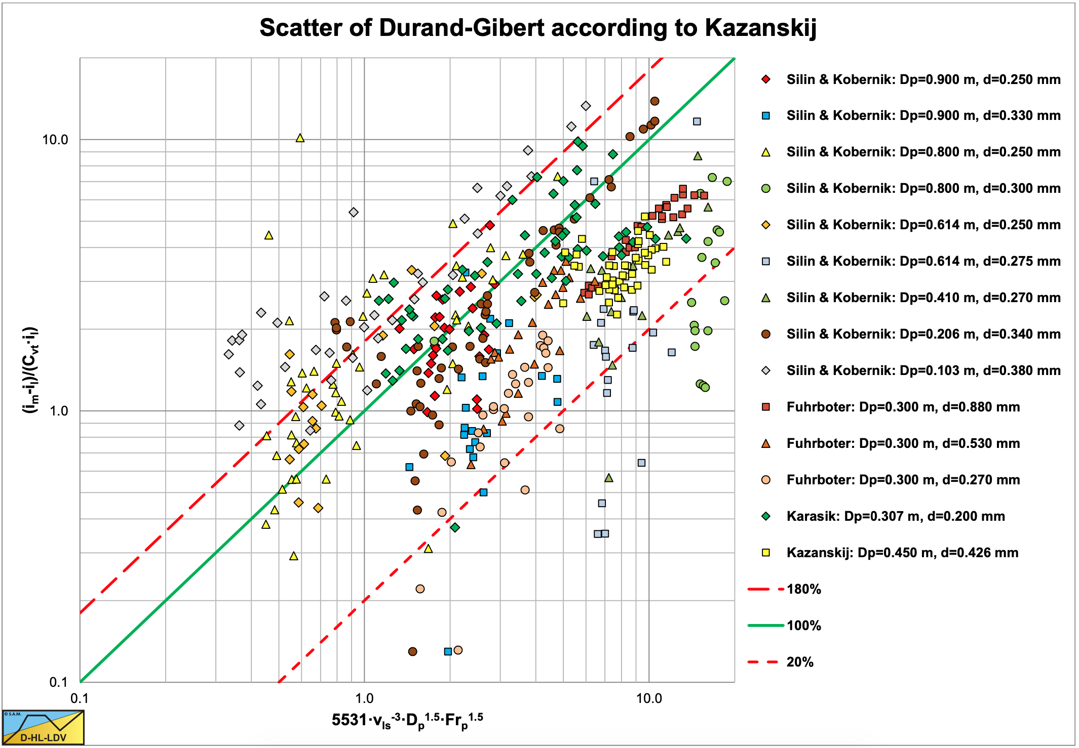
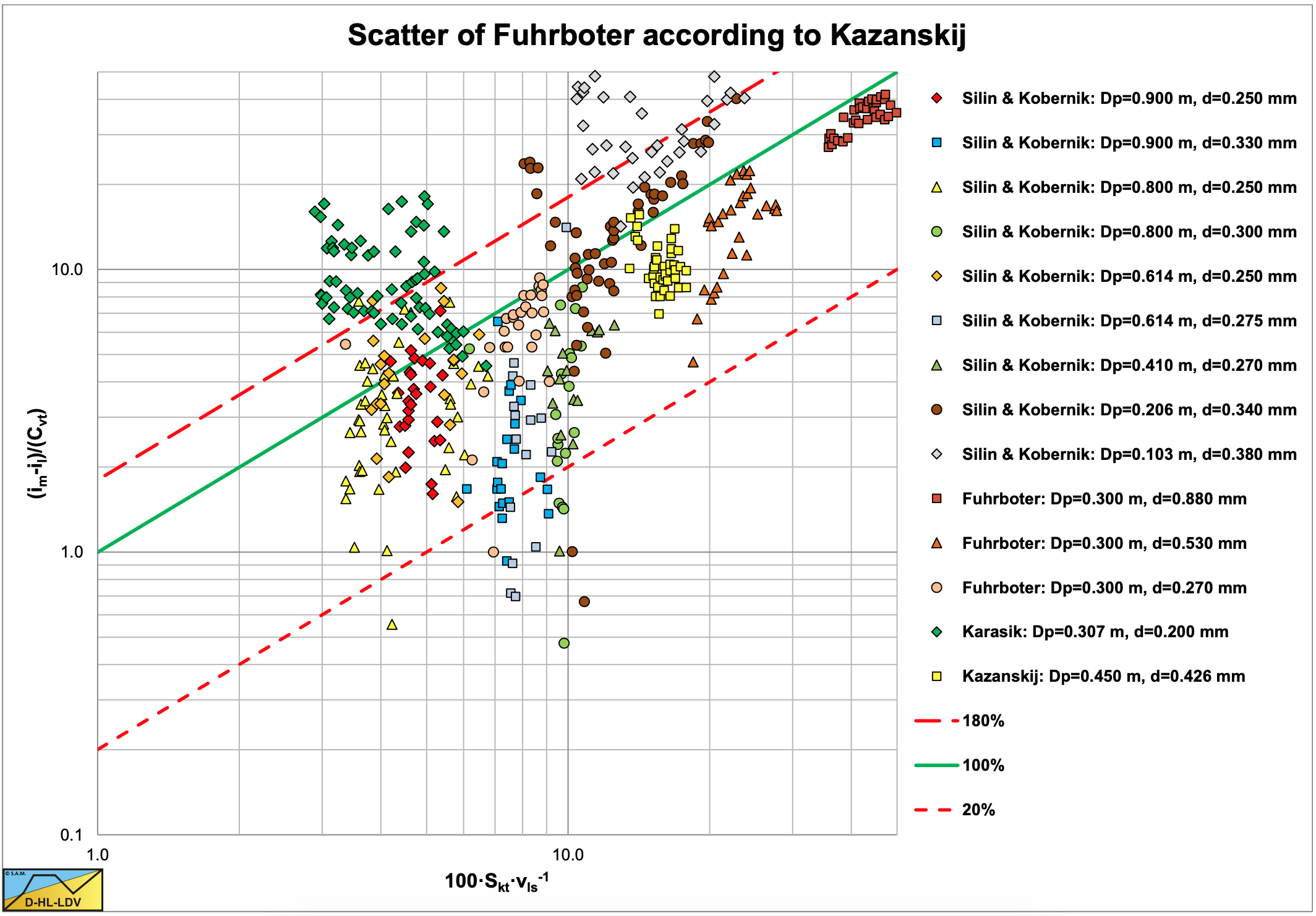
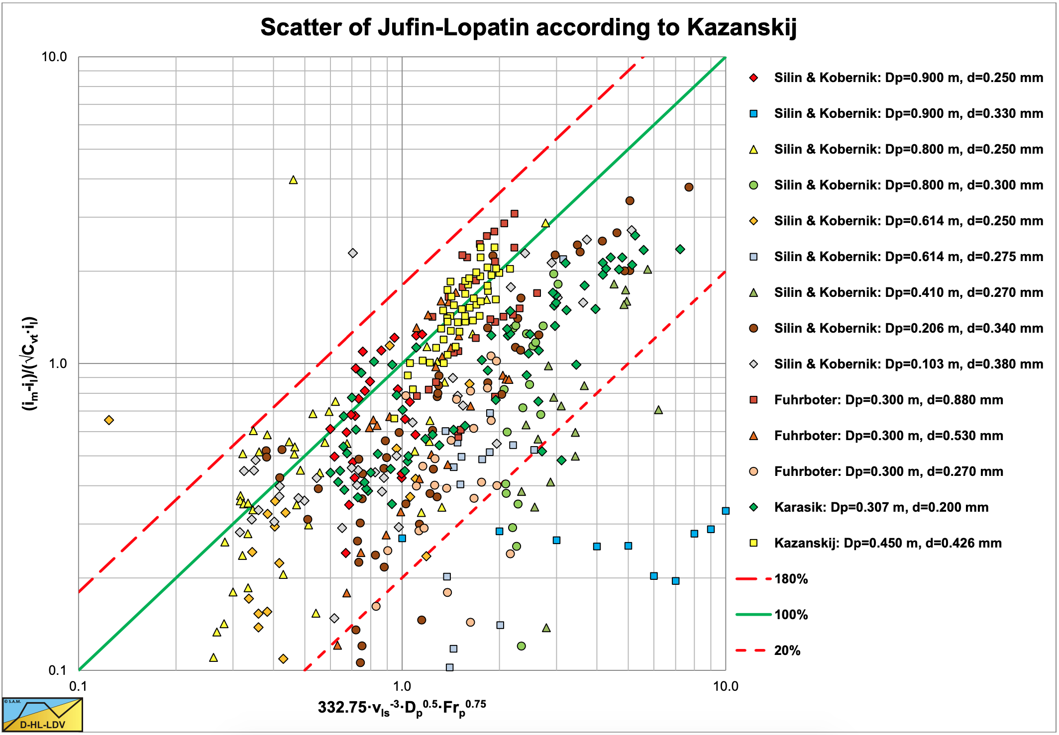
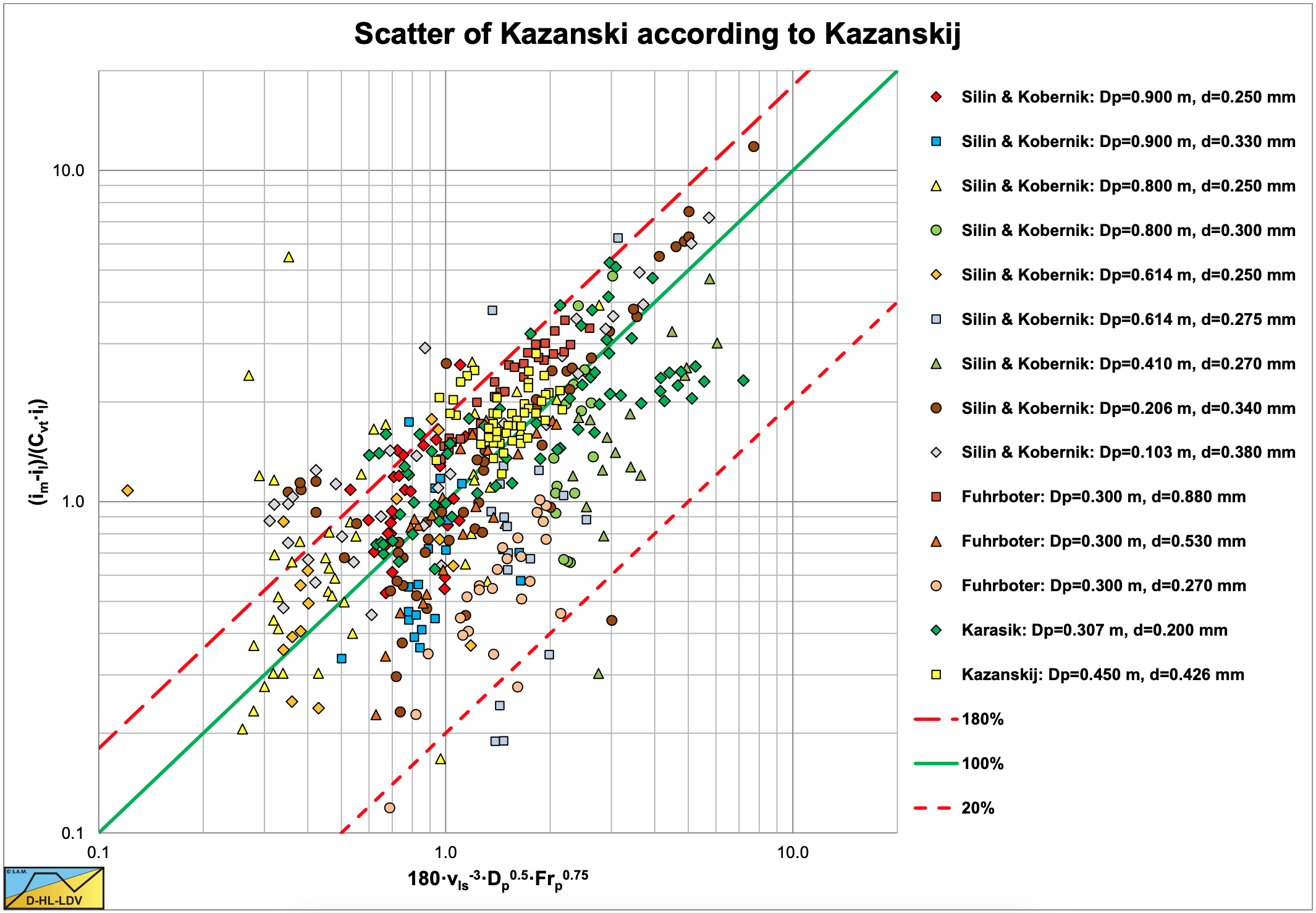
\(\newcommand{\avec}{\mathbf a}\) \(\newcommand{\bvec}{\mathbf b}\) \(\newcommand{\cvec}{\mathbf c}\) \(\newcommand{\dvec}{\mathbf d}\) \(\newcommand{\dtil}{\widetilde{\mathbf d}}\) \(\newcommand{\evec}{\mathbf e}\) \(\newcommand{\fvec}{\mathbf f}\) \(\newcommand{\nvec}{\mathbf n}\) \(\newcommand{\pvec}{\mathbf p}\) \(\newcommand{\qvec}{\mathbf q}\) \(\newcommand{\svec}{\mathbf s}\) \(\newcommand{\tvec}{\mathbf t}\) \(\newcommand{\uvec}{\mathbf u}\) \(\newcommand{\vvec}{\mathbf v}\) \(\newcommand{\wvec}{\mathbf w}\) \(\newcommand{\xvec}{\mathbf x}\) \(\newcommand{\yvec}{\mathbf y}\) \(\newcommand{\zvec}{\mathbf z}\) \(\newcommand{\rvec}{\mathbf r}\) \(\newcommand{\mvec}{\mathbf m}\) \(\newcommand{\zerovec}{\mathbf 0}\) \(\newcommand{\onevec}{\mathbf 1}\) \(\newcommand{\real}{\mathbb R}\) \(\newcommand{\twovec}[2]{\left[\begin{array}{r}#1 \\ #2 \end{array}\right]}\) \(\newcommand{\ctwovec}[2]{\left[\begin{array}{c}#1 \\ #2 \end{array}\right]}\) \(\newcommand{\threevec}[3]{\left[\begin{array}{r}#1 \\ #2 \\ #3 \end{array}\right]}\) \(\newcommand{\cthreevec}[3]{\left[\begin{array}{c}#1 \\ #2 \\ #3 \end{array}\right]}\) \(\newcommand{\fourvec}[4]{\left[\begin{array}{r}#1 \\ #2 \\ #3 \\ #4 \end{array}\right]}\) \(\newcommand{\cfourvec}[4]{\left[\begin{array}{c}#1 \\ #2 \\ #3 \\ #4 \end{array}\right]}\) \(\newcommand{\fivevec}[5]{\left[\begin{array}{r}#1 \\ #2 \\ #3 \\ #4 \\ #5 \\ \end{array}\right]}\) \(\newcommand{\cfivevec}[5]{\left[\begin{array}{c}#1 \\ #2 \\ #3 \\ #4 \\ #5 \\ \end{array}\right]}\) \(\newcommand{\mattwo}[4]{\left[\begin{array}{rr}#1 \amp #2 \\ #3 \amp #4 \\ \end{array}\right]}\) \(\newcommand{\laspan}[1]{\text{Span}\{#1\}}\) \(\newcommand{\bcal}{\cal B}\) \(\newcommand{\ccal}{\cal C}\) \(\newcommand{\scal}{\cal S}\) \(\newcommand{\wcal}{\cal W}\) \(\newcommand{\ecal}{\cal E}\) \(\newcommand{\coords}[2]{\left\{#1\right\}_{#2}}\) \(\newcommand{\gray}[1]{\color{gray}{#1}}\) \(\newcommand{\lgray}[1]{\color{lightgray}{#1}}\) \(\newcommand{\rank}{\operatorname{rank}}\) \(\newcommand{\row}{\text{Row}}\) \(\newcommand{\col}{\text{Col}}\) \(\renewcommand{\row}{\text{Row}}\) \(\newcommand{\nul}{\text{Nul}}\) \(\newcommand{\var}{\text{Var}}\) \(\newcommand{\corr}{\text{corr}}\) \(\newcommand{\len}[1]{\left|#1\right|}\) \(\newcommand{\bbar}{\overline{\bvec}}\) \(\newcommand{\bhat}{\widehat{\bvec}}\) \(\newcommand{\bperp}{\bvec^\perp}\) \(\newcommand{\xhat}{\widehat{\xvec}}\) \(\newcommand{\vhat}{\widehat{\vvec}}\) \(\newcommand{\uhat}{\widehat{\uvec}}\) \(\newcommand{\what}{\widehat{\wvec}}\) \(\newcommand{\Sighat}{\widehat{\Sigma}}\) \(\newcommand{\lt}{<}\) \(\newcommand{\gt}{>}\) \(\newcommand{\amp}{&}\) \(\definecolor{fillinmathshade}{gray}{0.9}\)Kazanskij (1978) gave an overview of the state of the art of slurry head loss models up to 1978. He showed the models of Durand & Condolios (1952), Condolios & Chapus (1963A), Bonnington (1961), Chaskelberg & Karlin (1976), Ellis & Round (1963), Kazanskij (1967), Zandi & Govatos (1967), Babcock (1970), Welte (1971), Newitt et al. (1955), Jufin & Lopatin (1966), Silin & Kobernik (1962), Charles (1970), Worster (1955), Fuhrboter (1961), Korzajev (1964), Duckworth & Argyros (1972), Vocadlo (1972), Jufin (1965), Wiedenroth (1967), Brauer (1971), Karasik (1973), Smoldyrev (1970) and Krivenko (1970). Some of the researchers have different models for different flow regimes. Kazanskij (1978) selected 4 models to investigate the scatter of the experimental values of the hydraulic gradient versus the hydraulic gradient determined with the model equations. These 4 models are the model of Durand & Condolios (1952), the model of Fuhrboter (1961), the model of Jufin & Lopatin (1966) and the model of Kazanskij (1978).
Durand & Condolios (1952), Figure 6.14-1:
\[\ \mathrm{x}=\mathrm{1 8 0} \cdot \mathrm{F r}^{-3} \cdot \operatorname{Fr}_{\mathrm{x} \mathrm{D}}^{\mathrm{1 . 5}}=\mathrm{5 5 3 1} \cdot \frac{\mathrm{D}_{\mathrm{p}}^{\mathrm{1 . 5}} \cdot \mathrm{F r}_{\mathrm{x D}}^{\mathrm{1 . 5}}}{\mathrm{v}_{\mathrm{l s}}^{\mathrm{3}}} \quad\text{ and }\quad \mathrm{y}=\frac{\mathrm{i}_{\mathrm{m}}-\mathrm{i}_{\mathrm{l}}}{\mathrm{C}_{\mathrm{v t}} \cdot \mathrm{i}_{\mathrm{l}}}\]
Fuhrboter (1961), Figure 6.14-2:
\[\ \mathrm{x}=\mathrm{1 0 0} \cdot \frac{\mathrm{S}_{\mathrm{k t}}}{\mathrm{v}_{\mathrm{l s}}}=\mathrm{1 0 0} \cdot \frac{\mathrm{2 .5 9} \cdot \mathrm{d}-\mathrm{0 .3 7}}{\mathrm{v}_{\mathrm{l s}}} \quad\text{ and }\quad \mathrm{y}=\frac{\mathrm{i}_{\mathrm{m}}-\mathrm{i}_{\mathrm{l}}}{\mathrm{C}_{\mathrm{vt}}}\]
Miedema (2014) has shown that the slip ratio of 0.65 as used by Fuhrboter (1961) is not correct. Fuhrboter used the ratio of the propagation velocity of density waves to the line speed as a slip ratio. Since this factor, in the form of 1/0.65, is present in both the abscissa and the ordinate, this does not influence the correlation, but on both the abscissa and the ordinate the values should be multiplied by 0.65. Another minor issue is, that the abscissa and the ordinate are per 100 m of pipe length. This is important for the Fuhrboter graph, since the Fuhrboter equation does not contain a division by the hydraulic gradient, which means the ordinate is not dimensionless. For the other 3 models considered here the ordinates are dimensionless, so this issue does not play a role. From a reconstruction of the data points it also appeared that Kazanskij (1978) used the Skt values of a d=0.33 mm particle for the d=0.30 mm, Dp=0.8 m and d=0.275 mm, Dp=0.614 m particles.
Jufin * Lopatin (1966), Figure 6.14-3:
\[\ \mathrm{x}=332.75 \cdot \frac{\mathrm{D}_{\mathrm{p}}^{0.5} \cdot \mathrm{Fr}_{\mathrm{xJ}}^{0.75}}{\mathrm{v}_{\mathrm{ls}}^{3}} \quad\text{ and }\quad \mathrm{y}=\frac{\mathrm{i}_{\mathrm{m}}-\mathrm{i}_{\mathrm{l}}}{\sqrt{\mathrm{C}_{\mathrm{vt}}} \cdot \mathrm{i}_{\mathrm{l}}}\]
Kazanskij (1978), Figure 6.14-4:
\[\ \mathrm{x=180 \cdot \frac{D_{p}^{0.5} \cdot F r_{x J}^{0.75}}{v_{l s}^{3}} \quad\text{ and }\quad y=\frac{i_{m}-i_{l}}{C_{v t} \cdot i_{l}}}\]
Kazanskij (1978) remarks that the accuracy of experiments with concentrations below 8% is not very good. In his paper he shows graphs with and without the experiments below 8%. A general conclusion based on the 4 graphs is that the Jufin & Lopatin model gives the best correlation, especially for the large diameter pipes, which is of interest for the dredging industry. However Jufin & Lopatin also gives a lot of scatter, meaning that the parameters on the axis still do not cover the real slurry transport process.
Based on a reconstruction of the hydraulic gradients versus line speeds, it should be concluded that most data points are in the (pseudo) homogeneous flow regime, except for the very small pipe diameters. The graphs of this reconstruction can be found on www.dhlldv.com.
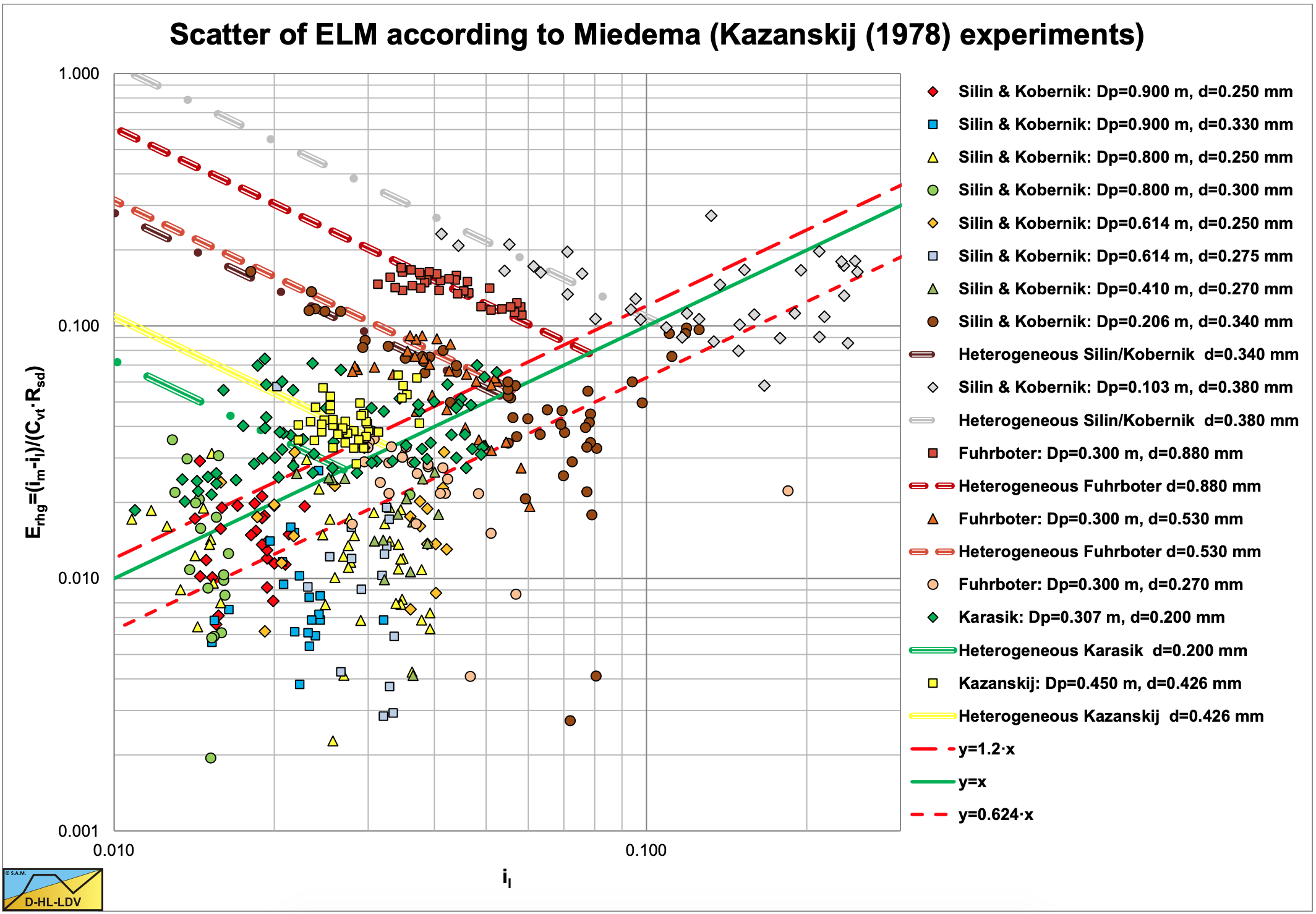
For all the models 100% means a perfect fit. The other two lines give +/- 80%.
Since many data points are in between the Equivalent Liquid Method (ELM) curve and the liquid curve, it is interesting to create a graph showing the data points compared to the ELM method. The graph with the relative excess hydraulic gradient Erhg versus the liquid hydraulic gradient il is suitable for this. Figure 6.14-5 shows this graph. The ELM curve is the curve y=x. The graph shows that some experiments were in the heterogeneous region, in which case the heterogeneous curve is also drawn. For the data points below 120% (arbitrary) of the ELM curve, the average ratio is determined, resulting in a factor of 0.624. Below 100% this ratio is 0.55. Below 130% this ratio is 0.67. This means that on average the data points in the homogeneous regime follow 62.4% of the ELM curve. This is close to the 60% as mentioned by Newitt et al. (1955). Miedema (2015) gives a possible explanation for this reduction based on the assumption of a watery viscous sub layer.
From this analysis it is clear that different regimes should not be mixed in one equation. Heterogeneous and homogeneous regimes have a different behavior and require different models.
The relative excess hydraulic gradient Erhg is:
\[\ \mathrm{E}_{\mathrm{r h g}}=\left(\frac{\mathrm{i}_{\mathrm{m}}-\mathrm{i}_{\mathrm{l}}}{\mathrm{R}_{\mathrm{s d}} \cdot \mathrm{C}_{\mathrm{v t}}}\right)\]
The liquid hydraulic gradient il is:
\[\ \mathrm{i_{l}}=\frac{\Delta \mathrm{p}}{\rho_{\mathrm{l}} \cdot \mathrm{g} \cdot \Delta \mathrm{L}}=\frac{\lambda_{\mathrm{l}} \cdot \mathrm{v}_{\mathrm{ls}}^{2}}{\mathrm{2} \cdot \mathrm{g} \cdot \mathrm{D}_{\mathrm{p}}}\]
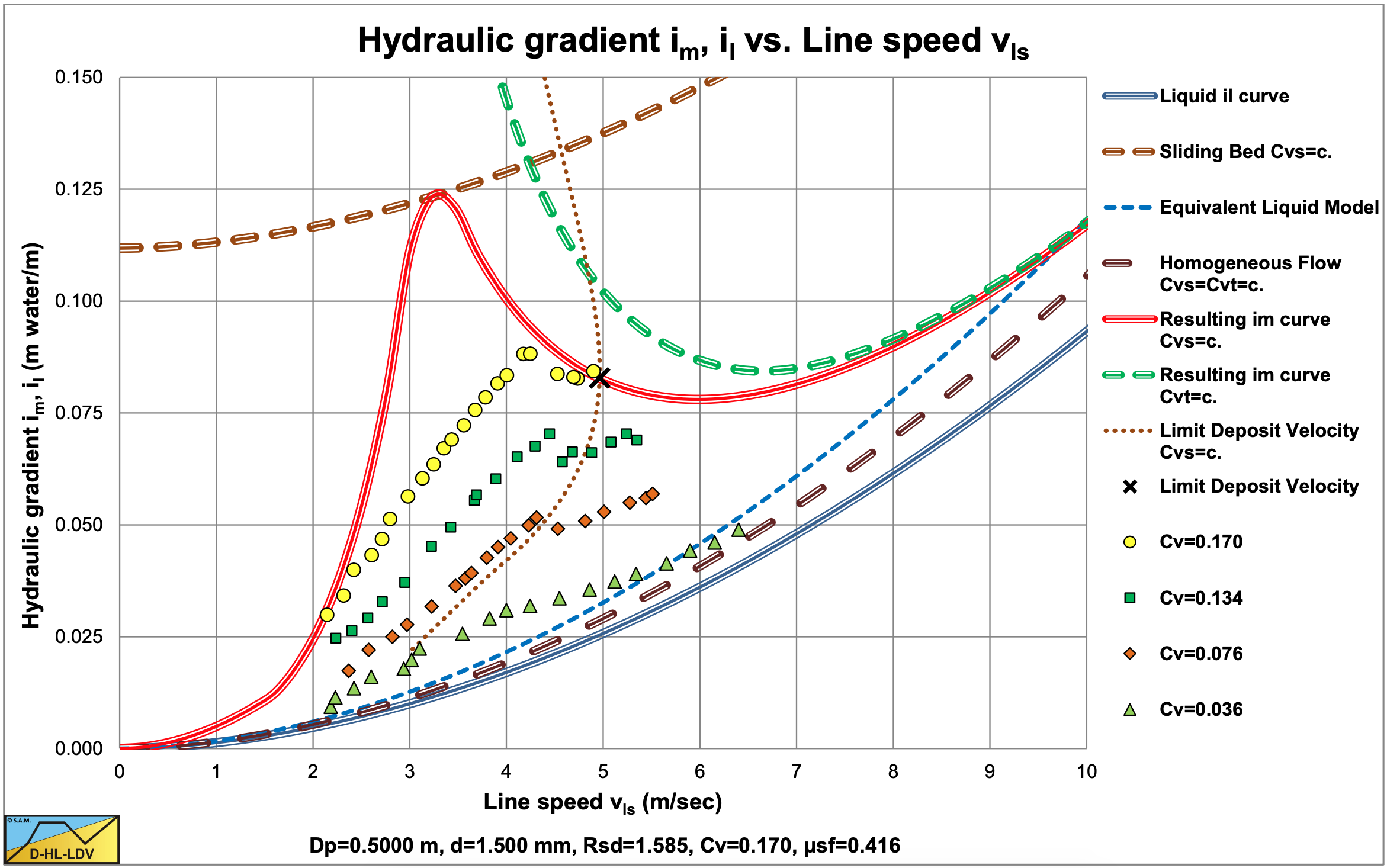
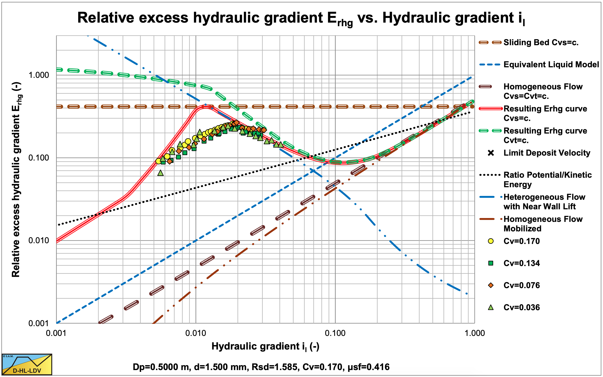
Kazanskij (1980) carried out experiments in a Dp=0.5 m pipe with d=1.5 mm particles. The results are shown in Figure 6.14-6 and Figure 6.14-7. The experiments were carried out with constant spatial volumetric concentration, which is also clear from the figures. Most experiments were below the LDV. The value of these experiments is the transition behavior from the fixed bed to the heterogeneous regime, which is more smooth than the DHLLDV Framework prediction. For normal dredging operations this is not very relevant, since most operations are above the LDV, however from a scientific point of view it is.