
6.10: The Turian and Yuan (1977) Fit Model
- Page ID
- 31042

\( \newcommand{\vecs}[1]{\overset { \scriptstyle \rightharpoonup} {\mathbf{#1}} } \)
\( \newcommand{\vecd}[1]{\overset{-\!-\!\rightharpoonup}{\vphantom{a}\smash {#1}}} \)
\( \newcommand{\id}{\mathrm{id}}\) \( \newcommand{\Span}{\mathrm{span}}\)
( \newcommand{\kernel}{\mathrm{null}\,}\) \( \newcommand{\range}{\mathrm{range}\,}\)
\( \newcommand{\RealPart}{\mathrm{Re}}\) \( \newcommand{\ImaginaryPart}{\mathrm{Im}}\)
\( \newcommand{\Argument}{\mathrm{Arg}}\) \( \newcommand{\norm}[1]{\| #1 \|}\)
\( \newcommand{\inner}[2]{\langle #1, #2 \rangle}\)
\( \newcommand{\Span}{\mathrm{span}}\)
\( \newcommand{\id}{\mathrm{id}}\)
\( \newcommand{\Span}{\mathrm{span}}\)
\( \newcommand{\kernel}{\mathrm{null}\,}\)
\( \newcommand{\range}{\mathrm{range}\,}\)
\( \newcommand{\RealPart}{\mathrm{Re}}\)
\( \newcommand{\ImaginaryPart}{\mathrm{Im}}\)
\( \newcommand{\Argument}{\mathrm{Arg}}\)
\( \newcommand{\norm}[1]{\| #1 \|}\)
\( \newcommand{\inner}[2]{\langle #1, #2 \rangle}\)
\( \newcommand{\Span}{\mathrm{span}}\) \( \newcommand{\AA}{\unicode[.8,0]{x212B}}\)
\( \newcommand{\vectorA}[1]{\vec{#1}} % arrow\)
\( \newcommand{\vectorAt}[1]{\vec{\text{#1}}} % arrow\)
\( \newcommand{\vectorB}[1]{\overset { \scriptstyle \rightharpoonup} {\mathbf{#1}} } \)
\( \newcommand{\vectorC}[1]{\textbf{#1}} \)
\( \newcommand{\vectorD}[1]{\overrightarrow{#1}} \)
\( \newcommand{\vectorDt}[1]{\overrightarrow{\text{#1}}} \)
\( \newcommand{\vectE}[1]{\overset{-\!-\!\rightharpoonup}{\vphantom{a}\smash{\mathbf {#1}}}} \)
\( \newcommand{\vecs}[1]{\overset { \scriptstyle \rightharpoonup} {\mathbf{#1}} } \)
\( \newcommand{\vecd}[1]{\overset{-\!-\!\rightharpoonup}{\vphantom{a}\smash {#1}}} \)
\(\newcommand{\avec}{\mathbf a}\) \(\newcommand{\bvec}{\mathbf b}\) \(\newcommand{\cvec}{\mathbf c}\) \(\newcommand{\dvec}{\mathbf d}\) \(\newcommand{\dtil}{\widetilde{\mathbf d}}\) \(\newcommand{\evec}{\mathbf e}\) \(\newcommand{\fvec}{\mathbf f}\) \(\newcommand{\nvec}{\mathbf n}\) \(\newcommand{\pvec}{\mathbf p}\) \(\newcommand{\qvec}{\mathbf q}\) \(\newcommand{\svec}{\mathbf s}\) \(\newcommand{\tvec}{\mathbf t}\) \(\newcommand{\uvec}{\mathbf u}\) \(\newcommand{\vvec}{\mathbf v}\) \(\newcommand{\wvec}{\mathbf w}\) \(\newcommand{\xvec}{\mathbf x}\) \(\newcommand{\yvec}{\mathbf y}\) \(\newcommand{\zvec}{\mathbf z}\) \(\newcommand{\rvec}{\mathbf r}\) \(\newcommand{\mvec}{\mathbf m}\) \(\newcommand{\zerovec}{\mathbf 0}\) \(\newcommand{\onevec}{\mathbf 1}\) \(\newcommand{\real}{\mathbb R}\) \(\newcommand{\twovec}[2]{\left[\begin{array}{r}#1 \\ #2 \end{array}\right]}\) \(\newcommand{\ctwovec}[2]{\left[\begin{array}{c}#1 \\ #2 \end{array}\right]}\) \(\newcommand{\threevec}[3]{\left[\begin{array}{r}#1 \\ #2 \\ #3 \end{array}\right]}\) \(\newcommand{\cthreevec}[3]{\left[\begin{array}{c}#1 \\ #2 \\ #3 \end{array}\right]}\) \(\newcommand{\fourvec}[4]{\left[\begin{array}{r}#1 \\ #2 \\ #3 \\ #4 \end{array}\right]}\) \(\newcommand{\cfourvec}[4]{\left[\begin{array}{c}#1 \\ #2 \\ #3 \\ #4 \end{array}\right]}\) \(\newcommand{\fivevec}[5]{\left[\begin{array}{r}#1 \\ #2 \\ #3 \\ #4 \\ #5 \\ \end{array}\right]}\) \(\newcommand{\cfivevec}[5]{\left[\begin{array}{c}#1 \\ #2 \\ #3 \\ #4 \\ #5 \\ \end{array}\right]}\) \(\newcommand{\mattwo}[4]{\left[\begin{array}{rr}#1 \amp #2 \\ #3 \amp #4 \\ \end{array}\right]}\) \(\newcommand{\laspan}[1]{\text{Span}\{#1\}}\) \(\newcommand{\bcal}{\cal B}\) \(\newcommand{\ccal}{\cal C}\) \(\newcommand{\scal}{\cal S}\) \(\newcommand{\wcal}{\cal W}\) \(\newcommand{\ecal}{\cal E}\) \(\newcommand{\coords}[2]{\left\{#1\right\}_{#2}}\) \(\newcommand{\gray}[1]{\color{gray}{#1}}\) \(\newcommand{\lgray}[1]{\color{lightgray}{#1}}\) \(\newcommand{\rank}{\operatorname{rank}}\) \(\newcommand{\row}{\text{Row}}\) \(\newcommand{\col}{\text{Col}}\) \(\renewcommand{\row}{\text{Row}}\) \(\newcommand{\nul}{\text{Nul}}\) \(\newcommand{\var}{\text{Var}}\) \(\newcommand{\corr}{\text{corr}}\) \(\newcommand{\len}[1]{\left|#1\right|}\) \(\newcommand{\bbar}{\overline{\bvec}}\) \(\newcommand{\bhat}{\widehat{\bvec}}\) \(\newcommand{\bperp}{\bvec^\perp}\) \(\newcommand{\xhat}{\widehat{\xvec}}\) \(\newcommand{\vhat}{\widehat{\vvec}}\) \(\newcommand{\uhat}{\widehat{\uvec}}\) \(\newcommand{\what}{\widehat{\wvec}}\) \(\newcommand{\Sighat}{\widehat{\Sigma}}\) \(\newcommand{\lt}{<}\) \(\newcommand{\gt}{>}\) \(\newcommand{\amp}{&}\) \(\definecolor{fillinmathshade}{gray}{0.9}\)6.13.1 Introduction
Turian & Yuan (1977) developed pressure drop correlations for flow of slurries in pipelines for 4 flow regimes. They defined flow with a stationary bed, saltation flow, heterogeneous flow and homogeneous flow. No distinctions have been made for sliding bed flow and sheet flow, so these regimes are part of the 4 regimes defined. A total number of 2848 data points were used to find correlations for each of the 4 regimes. For the stationary bed regime 361 data points were used, for the saltation regime 1230 data points, for the heterogeneous regime 493 data points and for the homogeneous regime 645 data points. The data points are from experiments with a pipe diameter Dp from 0.0126 m to 0.7 m , a relative submerged density Rsd from 0.16 to 10.3, a particle size d from 0.03 mm to 38 mm, a solids concentration Cv from 0% to 42% and a mean line speed vls from 0 m/sec to 6.7 m/sec. It should be mentioned however that most of the experiments were carried out with sand or glass and only 16 data points were found from pipe diameters above 15 cm. Turian & Yuan (1977) correlated the pressure losses to a set of 4 parameters, the volumetric concentration Cv, the Fanning friction factor f, the particle drag coefficient CD and the flow Froude number Fr. It is not always clear whether the spatial or the transport concentration is used in the equation, but based on an analysis of the resulting equation it is assumed to be the transport concentration. In the original equations of Turian & Yuan (1977), they used the concentration as a percentage. In the equations as found later and as presented here, the concentration is used as a fraction. The result is that all the proportionality coefficients had to be multiplied by 100 to the power of the concentration.
The drag coefficient for the terminal settling velocity CD is:
\[\ \mathrm{C_{D}=\frac{4}{3} \cdot \frac{R_{s d} \cdot g \cdot d}{v_{t}^{2}}}\]
The Froude number Fr of the flow in the Turian & Yuan (1977) equations is:
\[\ \mathrm{F r}=\frac{\mathrm{v}_{\mathrm{l} \mathrm{s}}^{2}}{\mathrm{R}_{\mathrm{s d}} \cdot \mathrm{g} \cdot \mathrm{D}_{\mathrm{p}}}\]
The pressure losses of a liquid can be calculated with:
\[\ \Delta \mathrm{p}_{\mathrm{l}}=\mathrm{2} \cdot \mathrm{f}_{\mathrm{l}} \cdot \rho_{\mathrm{l}} \cdot \mathrm{v}_{\mathrm{l} \mathrm{s}}^{2} \cdot \frac{\Delta \mathrm{L}}{\mathrm{D}_{\mathrm{p}}}=\lambda_{\mathrm{l}} \cdot \frac{\mathrm{1}}{2} \cdot \rho_{\mathrm{l}} \cdot \mathrm{v}_{\mathrm{l s}}^{2} \cdot \frac{\Delta \mathrm{L}}{\mathrm{D}_{\mathrm{p}}}\]
The pressure losses of a mixture can be calculated with:
\[\ \Delta \mathrm{p}_{\mathrm{m}}=\mathrm{2} \cdot \mathrm{f}_{\mathrm{m}} \cdot \rho_{\mathrm{l}} \cdot \mathrm{v}_{\mathrm{l} \mathrm{s}}^{2} \cdot \frac{\Delta \mathrm{L}}{\mathrm{D}_{\mathrm{p}}}=\lambda_{\mathrm{m}} \cdot \frac{\mathrm{1}}{2} \cdot \rho_{\mathrm{l}} \cdot \mathrm{v}_{\mathrm{l} \mathrm{s}}^{2} \cdot \frac{\Delta \mathrm{L}}{\mathrm{D}_{\mathrm{p}}}\]
The general solids excess pressure equation of Turian & Yuan has the following form:
\[\ \begin{array}{left} \mathrm{f}_{\mathrm{m}}-\mathrm{f}_{\mathrm{l}}=\frac{\lambda_{\mathrm{m}}}{\mathrm{4}}-\frac{\lambda_{\mathrm{l}}}{\mathrm{4}}=\mathrm{K} \cdot \mathrm{C}_{\mathrm{v}}^{\mathrm{\alpha}} \cdot \mathrm{f}_{\mathrm{l}}^{\boldsymbol{\beta}} \cdot\left(\frac{\mathrm{4}}{\mathrm{3}} \cdot \frac{\mathrm{R}_{\mathrm{s} \mathrm{d}} \cdot \mathrm{g} \cdot \mathrm{d}}{\mathrm{v}_{\mathrm{t}}^{2}}\right)^{\gamma} \cdot\left(\frac{\mathrm{v}_{\mathrm{l} \mathrm{s}}^{2}}{\mathrm{R}_{\mathrm{s d}} \cdot \mathrm{g} \cdot \mathrm{D}_{\mathrm{p}}}\right)^{\mathrm{\delta}}\\
\mathrm{f}_{\mathrm{m}}-\mathrm{f}_{\mathrm{l}}=\frac{\lambda_{\mathrm{m}}}{\mathrm{4}}-\frac{\lambda_{\mathrm{l}}}{\mathrm{4}}=\mathrm{K} \cdot \mathrm{C}_{\mathrm{v}}^{\alpha} \cdot \mathrm{f}_{\mathrm{l}}^{\beta} \cdot \mathrm{C}_{\mathrm{D}}^{\gamma} \cdot \mathrm{F} \mathrm{r}^{\delta}\end{array}\]
The proportionality coefficient K and the powers α, β, γ and δ are determined for each of the 4 flow regimes by correlation techniques. It should be mentioned that the form of this equation limits the possible combinations between the parameters and also the fact that the solids effect is described by one single term limits the physics behind the model.
6.13.2 The Regime Equations
The friction coefficient fm depends on the regime according to:
Fixed bed/sliding bed, regime 0:
\[\ \mathrm{f_{m}-f_{l}=\frac{\lambda_{m}}{4}-\frac{\lambda_{l}}{4}=12.13 \cdot C_{v}^{0.7389} \cdot\left(\frac{\lambda_{l}}{4}\right)^{0.7717} \cdot C_{D}^{-0.4054} \cdot F r^{-1.096}}\]
Saltation, regime 1:
\[\ \mathrm{f_{m}-f_{l}=\frac{\lambda_{m}}{4}-\frac{\lambda_{l}}{4}=107.1 \cdot C_{v}^{1.018} \cdot\left(\frac{\lambda_{l}}{4}\right)^{1.046} \cdot C_{D}^{-0.4213} \cdot F r^{-1.354}}\]
Heterogeneous suspension, regime 2:
\[\ \mathrm{f_{m}-f_{l}=\frac{\lambda_{m}}{4}-\frac{\lambda_{l}}{4}=30.11 \cdot C_{v}^{0.8687} \cdot\left(\frac{\lambda_{l}}{4}\right)^{1.200} \cdot C_{D}^{-0.1677} \cdot F r^{-0.6938}}\]
Homogeneous suspension, regime 3:
\[\ \mathrm{f_{m}-f_{l}=\frac{\lambda_{m}}{4}-\frac{\lambda_{l}}{4}=8.538 \cdot C_{v}^{0.5028} \cdot\left(\frac{\lambda_{l}}{4}\right)^{1.428} \cdot C_{D}^ {0.1516} \cdot F r^{-0.3531}}\]
6.13.3 Usage of the Equations
The Fanning friction factor for pure liquid transport can be written as:
\[\ \mathrm{f}_{\mathrm{l}}=\frac{\Delta \mathrm{p}_{\mathrm{l}}}{\mathrm{2} \cdot \rho_{\mathrm{l}} \cdot \mathrm{v}_{\mathrm{l} \mathrm{s}}^{2} \cdot \frac{\Delta \mathrm{L}}{\mathrm{D}_{\mathrm{p}}}}=\frac{\lambda_{\mathrm{l}}}{\mathrm{4}}\]
The Fanning friction factor for mixture transport can be written as:
\[\ \mathrm{f}_{\mathrm{m}}=\frac{\Delta \mathrm{p}_{\mathrm{m}}}{2 \cdot \rho_{\mathrm{l}} \cdot \mathrm{v}_{\mathrm{l} \mathrm{s}}^{2} \cdot \frac{\Delta \mathrm{L}}{\mathrm{D}_{\mathrm{p}}}}=\frac{\lambda_{\mathrm{m}}}{4}\]
Thus:
\[\ \begin{array}{left} \mathrm{f_{m}-f_{l}=\frac{\lambda_{m}}{4}-\frac{\lambda_{l}}{4}=\frac{\Delta p_{m}-\Delta p_{l}}{2 \cdot \rho_{l} \cdot v_{l s}^{2} \cdot \frac{\Delta L}{D_{p}}}=\frac{\left(\Delta p_{m}-\Delta p_{l}\right) \cdot D_{p}}{2 \cdot \rho_{l} \cdot v_{l s}^{2} \cdot \Delta L}}\\
\mathrm{f_{m}-f_{l}=\frac{\lambda_{m}}{4}-\frac{\lambda_{I}}{4}=\frac{\left(i_{m}-i_{l}\right) \cdot \rho_{l} \cdot g \cdot \Delta L}{2 \cdot \rho_{l} \cdot v_{l s}^{2} \cdot \frac{\Delta L}{D_{p}}}=\frac{\left(i_{m}-i_{l}\right) \cdot g \cdot D_{p}}{2 \cdot v_{l s}^{2}}}\end{array}\]
Or:
\[\ \begin{array}{left}\Delta \mathrm{p}_{\mathrm{m}}-\Delta \mathrm{p}_{\mathrm{l}}=\left(\mathrm{f}_{\mathrm{m}}-\mathrm{f}_{\mathrm{l}}\right) \cdot \frac{\mathrm{2} \cdot \mathrm{\rho}_{\mathrm{l}} \cdot \mathrm{v}_{\mathrm{l} \mathrm{s}}^{\mathrm{2}} \cdot \Delta \mathrm{L}}{\mathrm{D}_{\mathrm{p}}}=\left(\lambda_{\mathrm{m}}-\lambda_{\mathrm{l}}\right) \cdot \frac{\rho_{\mathrm{l}} \cdot \mathrm{v}_{\mathrm{ls}}^{\mathrm{2}} \cdot \mathrm{\Delta} \mathrm{L}}{\mathrm{2} \cdot \mathrm{D}_{\mathrm{p}}}\\
\mathrm{i}_{\mathrm{m}}-\mathrm{i}_{\mathrm{l}}=\left(\mathrm{f}_{\mathrm{m}}-\mathrm{f}_{\mathrm{l}}\right) \cdot \frac{\mathrm{2} \cdot \mathrm{v}_{\mathrm{l} \mathrm{s}}^{2}}{\mathrm{g} \cdot \mathrm{D}_{\mathrm{p}}}=\left(\lambda_{\mathrm{m}}-\lambda_{\mathrm{l}}\right) \cdot \frac{\mathrm{v}_{\mathrm{ls}}^{2}}{\mathrm{2} \cdot \mathrm{g} \cdot \mathrm{D}_{\mathrm{p}}}\end{array}\]
With the Froude number according to equation (6.13-2), the hydraulic gradient can be written as:
\[\ \mathrm{i}_{\mathrm{m}}-\mathrm{i}_{\mathrm{l}}=\left(\mathrm{f}_{\mathrm{m}}-\mathrm{f}_{\mathrm{l}}\right) \cdot \frac{\mathrm{2} \cdot \mathrm{v}_{\mathrm{l}}^{\mathrm{2}}}{\mathrm{g} \cdot \mathrm{D}_{\mathrm{p}}}=\left(\mathrm{f}_{\mathrm{m}}-\mathrm{f}_{\mathrm{l}}\right) \cdot \mathrm{2} \cdot \mathrm{R}_{\mathrm{s d}} \cdot \frac{\mathrm{v}_{\mathrm{ls}}^{\mathrm{2}}}{\mathrm{R}_{\mathrm{s d}} \cdot \mathrm{g} \cdot \mathrm{D}_{\mathrm{p}}}=\left(\mathrm{f}_{\mathrm{m}}-\mathrm{f}_{\mathrm{l}}\right) \cdot \mathrm{2} \cdot \mathrm{R}_{\mathrm{s d}} \cdot \mathrm{F} \mathrm{r}\]
The relative excess hydraulic gradient Erhg is now:
\[\ \mathrm{E}_{\mathrm{rhg}}=\frac{\left(\mathrm{i}_{\mathrm{m}}-\mathrm{i}_{\mathrm{l}}\right)}{\mathrm{R}_{\mathrm{s d}} \cdot \mathrm{C}_{\mathrm{v}}}=\frac{\left(\mathrm{f}_{\mathrm{m}}-\mathrm{f}_{\mathrm{l}}\right) \cdot \mathrm{2} \cdot \mathrm{F r}}{\mathrm{C}_{\mathrm{v}}}\]
In terms of the hydraulic gradient, the Turian & Yuan (1977) equations can be rewritten as:
Fixed bed/sliding bed, regime 0:
\[\ \left(\mathrm{i}_{\mathrm{m}}-\mathrm{i}_{\mathrm{l}}\right)=\mathrm{8 . 3 2 3} \cdot \mathrm{C}_{\mathrm{v}}^{\mathrm{0 . 7 3 8 9}} \cdot \lambda_{\mathrm{l}}^{0.7717} \cdot \mathrm{C}_{\mathrm{D}}^{-\mathrm{0 . 4 0 5 4} }\cdot \mathrm{F r}^{-\mathrm{0 . 0 9 6}} \cdot \mathrm{R}_{\mathrm{s d}}\]
Saltation, regime 1:
\[\ \left(\mathrm{i}_{\mathrm{m}}-\mathrm{i}_{\mathrm{l}}\right)=\mathrm{5 0 . 2 4} \cdot \mathrm{C}_{\mathrm{v}}^{\mathrm{1 . 0 1 8}} \cdot \lambda_{\mathrm{l}}^{\mathrm{1 . 0 4 6}} \cdot \mathrm{C _ { \mathrm { D } }}-\mathrm{0 . 4 2 1 3} \cdot \mathrm{F r}^{-\mathrm{0 . 3 5 4}} \cdot \mathrm{R}_{\mathrm{s d}}\]
Heterogeneous suspension, regime 2:
\[\ \left(\mathrm{i}_{\mathrm{m}}-\mathrm{i}_{\mathrm{l}}\right)=\mathrm{1 1 . 4 1} \cdot \mathrm{C}_{\mathrm{v}}^{\mathrm{0 . 8 6 8}} \cdot \lambda_{\mathrm{l}}^{\mathrm{1 . 2 0 0}} \cdot \mathrm{C _ { D }}^{-\mathrm{0 . 1 6 7 7}} \cdot \mathrm{F r}^{\mathrm{0 . 3 0 6 2}} \cdot \mathrm{R}_{\mathrm{s d}}\]
Homogeneous suspension, regime 3:
\[\ \left(\mathrm{i}_{\mathrm{m}}-\mathrm{i}_{\mathrm{l}}\right)=\mathrm{2 . 3 5 8} \cdot \mathrm{C}_{\mathrm{v}}^{\mathrm{0 . 5 0 2 8}} \cdot \lambda_{\mathrm{l}}^{\mathrm{1 . 4 2 8}} \cdot \mathrm{C _ { \mathrm { D } }}^{\mathrm{0 . 1 5 1 6}} \cdot \mathrm{F r}^{\mathrm{0 . 6 4 6 9}} \cdot \mathrm{R}_{\mathrm{s d}}\]
In terms of the Srs value, the Turian & Yuan (1977) equations can be rewritten as:
Fixed bed/sliding bed, regime 0:
\[\ \mathrm{E}_{\mathrm{r h g}}=\frac{\left(\mathrm{i}_{\mathrm{m}}-\mathrm{i}_{\mathrm{l}}\right)}{\mathrm{R}_{\mathrm{s d}} \cdot \mathrm{C}_{\mathrm{v}}}=\mathrm{8 . 3 2 3} \cdot \mathrm{C}_{\mathrm{v}}^{-\mathrm{0} . \mathrm{2 6 1 1}} \cdot \lambda_{\mathrm{l}}^{0.7717} \cdot \mathrm{C}_{\mathrm{D}}^{-\mathrm{0 . 4 0 5 4}} \cdot \mathrm{F r}^{-\mathrm{0 . 0 9 6}}\]
Saltation, regime 1:
\[\ \mathrm{E}_{\mathrm{r h g}}=\frac{\left(\mathrm{i}_{\mathrm{m}}-\mathrm{i}_{\mathrm{l}}\right)}{\mathrm{R}_{\mathrm{s d}} \cdot \mathrm{C}_{\mathrm{v}}}=\mathrm{5 0 . 2 4} \cdot \mathrm{C}_{\mathrm{v}}^{0.018} \cdot \lambda_{\mathrm{l}}^{\mathrm{1 . 0 4 6}} \cdot \mathrm{C}_{\mathrm{D}}^{-\mathrm{0 . 4 2 1 3}} \cdot \mathrm{F r}^{-\mathrm{0 . 3 5 4}}\]
Heterogeneous suspension, regime 2:
\[\ \mathrm{E}_{\mathrm{r h g}}=\frac{\left(\mathrm{i}_{\mathrm{m}}-\mathrm{i}_{\mathrm{l}}\right)}{\mathrm{R}_{\mathrm{s d}} \cdot \mathrm{C}_{\mathrm{v}}}=\mathrm{1 1 . 4 1} \cdot \mathrm{C}_{\mathrm{v}}^{-0.132} \cdot \lambda_{\mathrm{l}}^{\mathrm{1} .200} \cdot \mathrm{C}_{\mathrm{D}}^{-\mathrm{0 . 1 6 7 7}} \cdot \mathrm{F r}^{\mathrm{0 . 3 0 6 2}}\]
Homogeneous suspension, regime 3:
\[\ \mathrm{E}_{\mathrm{r h g}}=\frac{\left(\mathrm{i}_{\mathrm{m}}-\mathrm{i}_{\mathrm{l}}\right)}{\mathrm{R}_{\mathrm{s d}} \cdot \mathrm{C}_{\mathrm{v}}}=\mathrm{2 . 3 5 8} \cdot \mathrm{C}_{\mathrm{v}}^{-\mathrm{0 . 4 9 7 2}} \cdot \lambda_{\mathrm{l}}^{\mathrm{1 . 4 2 8}} \cdot \mathrm{C _ { D }}^{\mathrm{0 . 1 5 1 6}} \cdot \mathrm{F r}^{\mathrm{0 . 6 4 6 9}}\]
6.13.4 Analysis of the Turian & Yuan (1977) Equations
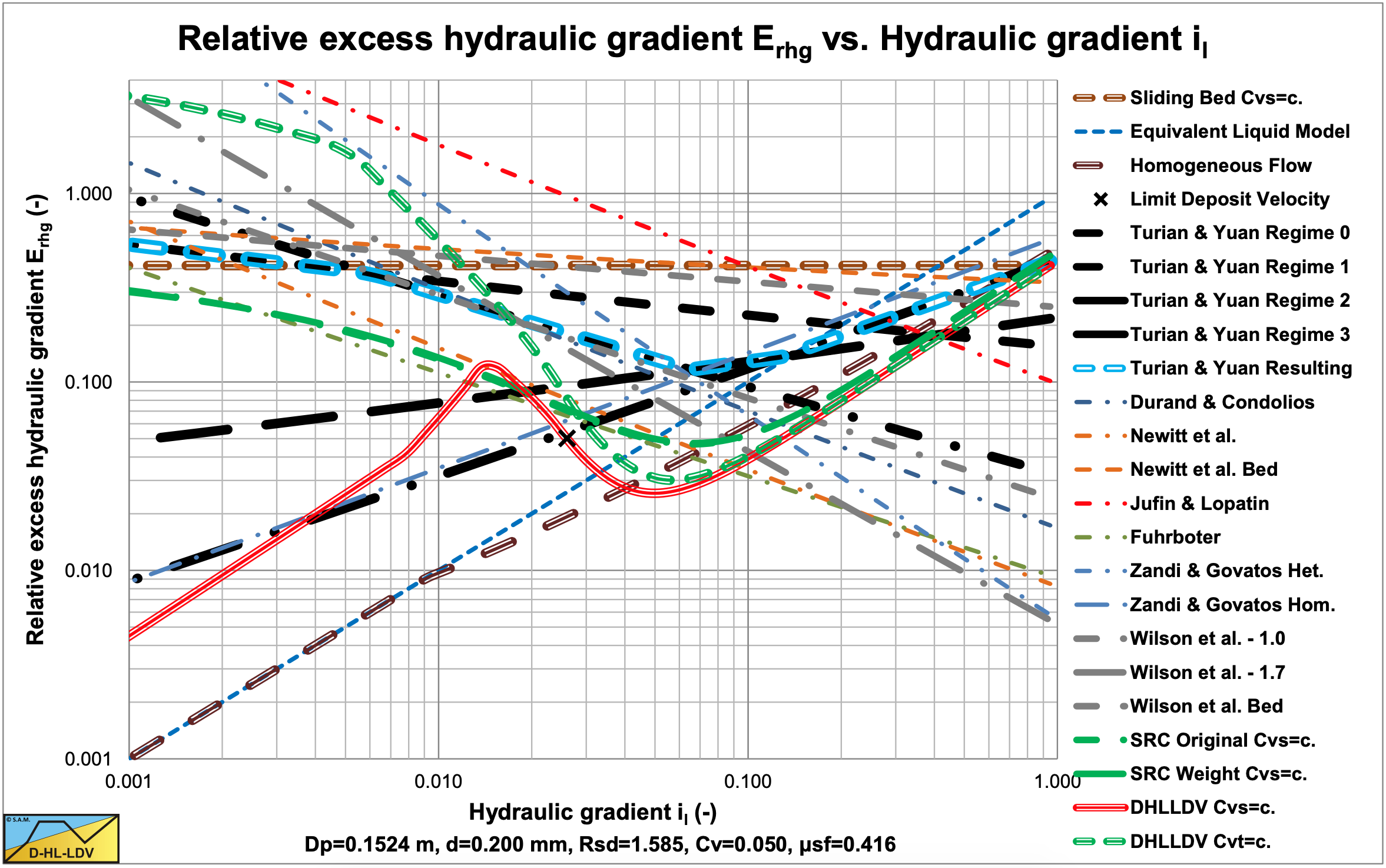
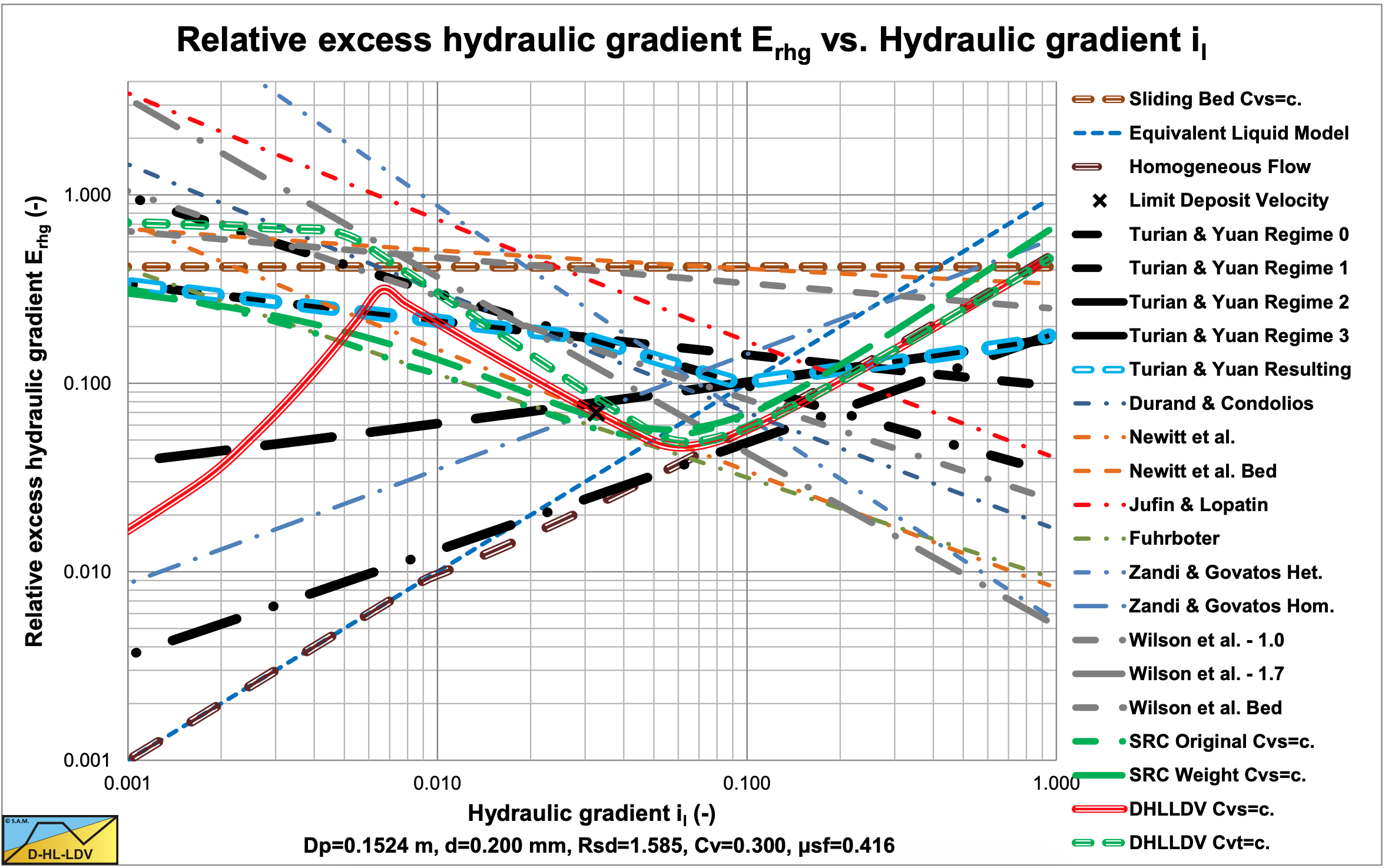
The Turian & Yuan (1977) correlation equations are based on one term for the solids effect of the pressure losses. In their equations they use the drag coefficient CD and the Froude number Fr, limiting the possible combinations of parameters. The relative submerged density Rsd, the particle diameter d and the terminal settling velocity vt are always present in a prescribed relation of the drag coefficient CD. The line speed vls, the relative submerged density Rsd and the pipe diameter Dp are presented in a prescribed relation in the Froude number. This limits the number of possible parameter combinations and also the absence of the sliding friction coefficient limits the explanation by real physics of the equations. For the analysis, the equations of Turian & Yuan (1977) are compared with the model of Miedema (2013S) as described in this book. This is illustrated in Figure 6.13-5 and Figure 6.13-6 for an 0.15 m pipe and a 0.2 mm particle.
Regime 0: Fixed bed or sliding bed, equation (6.13-20).
\[\ \mathrm{E}_{\mathrm{r h g}}=\frac{\left(\mathrm{i}_{\mathrm{m}}-\mathrm{i}_{\mathrm{l}}\right)}{\mathrm{R}_{\mathrm{s d}} \cdot \mathrm{C}_{\mathrm{v}}}=\mathrm{8 . 3 2 3 \cdot} \mathrm{C}_{\mathrm{v}}^{-\mathrm{0 . 2 6 1 1}}{ \cdot \lambda_{\mathrm{l}}^{\mathrm{0 . 7 7 1 7}} \cdot \mathrm{C}_{\mathrm{D}}^{-\mathrm{0 . 4 0 5 4}} \cdot \mathrm{F r}^{-\mathrm{0 . 0 9 6}}}\]
For the Erhg value, the fixed bed or sliding bed equation is almost independent of the Froude number, which points to a constant Erhg value as a function of the hydraulic gradient or of the line speed. A sliding bed however would require a sliding friction coefficient in the equation, which is absent. This may be compensated partly by the negative power of the drag coefficient, since smaller particles often have a smaller sliding friction coefficient. The negative power of the volumetric concentration can be explained. A power of 0 would be expected for a constant spatial volumetric concentration. A constant transport volumetric concentration would however result in a negative power. The positive power of the friction coefficient and the negative power of the drag coefficient can be explained by the liquid friction in the cross section above the bed. This liquid friction is the sum of the friction on the pipe wall and the friction on the bed. The drag coefficient is to some extent reversely proportional with the size of the bed particles, while the shear stress on the bed is proportional with the particle size. Figure 6.13-5 shows that the constant transport concentration model of Miedema (2013S) in the sliding bed region does not match the Turian & Yuan (1977) model exactly for a 5% concentration, but Figure 6.13-6 shows an almost perfect match if a sliding friction coefficient of 0.416 is applied. Since in both figures the Turian & Yuan (1977) curves decrease with an increasing hydraulic gradient, compared with horizontal curves according to Miedema (2013S) , the Turian & Yuan (1977) equations must be based on a constant volumetric transport (delivered) concentration.
Regime 1: Saltating transport, equation (6.13-21).
\[\ \mathrm{E}_{\mathrm{rhg}}=\frac{\left(\mathrm{i}_{\mathrm{m}}-\mathrm{i}_{\mathrm{l}}\right)}{\mathrm{R}_{\mathrm{s d}} \cdot \mathrm{C}_{\mathrm{v}}}=\mathrm{5 0 . 2 4} \cdot \mathrm{C}_{\mathrm{v}}^{\mathrm{0} . \mathrm{0 1 8}} \cdot \lambda_{\mathrm{l}}^{\mathrm{1 . 0 4 6}} \cdot \mathrm{C _ { D }}^{-\mathrm{0 . 4 2 1 3}} \cdot \mathrm{F r}^{-\mathrm{0 . 3 5 4}}\]
For the Erhg value, the saltating transport equation is almost independent of the volumetric concentration, just like the heterogeneous equation of Miedema (2013S). The saltating transport equation is almost proportional with the wall friction coefficient, giving a slight decrease of the Erhg value with increasing line speed. The proportionality with the CD value has a negative power of 0.4213, which means that smaller particles have less resistance. This proportionality is however much smaller than estimated by Durand & Condolios (1952), who found a power of 1.275. This power of 1.275 is also applied by Miedema (2013S) . The proportionality with the Froude number has a negative power of 0.354, which is small. This power results in a negative power for the line speed of 0.708, while most models use a negative power between 1 and 2 for the line speed. This small power may be the result of curve fitting over 3 regimes, the sliding bed regime, the heterogeneous regime and the pseudo homogeneous regime. At higher concentrations the heterogeneous regime maybe replaced by the sheet flow regime with a much smaller power
The saltating regime of Turian & Yuan (1977) seems to be more a combination of the heterogeneous regime and the sheet flow regime when it is compared to different other models.
The blue dashed lines show the resulting curves of Turian & Yuan (1977). The shape of these curves matches the shape of the DHLLDV Framework, however the values and the steepness do not match. Also a comparison with other models shows that most models show a much steeper curve compared to Turian & Yuan (1977) regime 1, which is supposed to be the heterogeneous regime.
Regime 2: Heterogeneous transport, equation (6.13-22).
\[\ \mathrm{E}_{\mathrm{r h g}}=\frac{\left(\mathrm{i}_{\mathrm{m}}-\mathrm{i}_{\mathrm{l}}\right)}{\mathrm{R}_{\mathrm{s d}} \cdot \mathrm{C}_{\mathrm{v}}}=\mathrm{1 1 . 4 1} \cdot \mathrm{C}_{\mathrm{v}}^{-\mathrm{0 . 1 3 2}} \cdot \lambda_{\mathrm{l}}^{\mathrm{1 . 2 0 0}} \cdot \mathrm{C _ { D }}^{-\mathrm{0 . 1 6 7 7}} \cdot \mathrm{F r}^{\mathrm{0 . 3 0 6 2}}\]
For the Erhg value, the heterogeneous transport equation is almost independent of the volumetric concentration, just like the heterogeneous equation of Miedema (2013S), although the Erhg will slightly decrease with increasing concentration. The heterogeneous transport equation is almost proportional with the wall friction coefficient, giving a slight decrease of the Erhg value with increasing line speed. The proportionality with the CD value has a negative power of 0.1677, which means that smaller particles have slightly less resistance, but this is a weak dependency. This proportionality is however much smaller than estimated by Durand & Condolios (1952), who found a power of 1.275 for heterogeneous transport. This power of 1.275 is also applied by Miedema (2013S). The proportionality with the Froude number has a positive power of 0.3062, which is small but this contradicts with all other models for heterogeneous transport which use a negative power between 1 and 2 for the line speed.
The heterogeneous regime of Turian & Yuan (1977) seems to be more a pseudo homogeneous regime or at the transition between heterogeneous and homogeneous regimes when it is compared to different other models.
Regime 3: Homogeneous transport, equation (6.13-23).
\[\ \mathrm{E}_{\mathrm{r h g}}=\frac{\left(\mathrm{i}_{\mathrm{m}}-\mathrm{i}_{\mathrm{l}}\right)}{\mathrm{R}_{\mathrm{s d}} \cdot \mathrm{C}_{\mathrm{v}}}=2.35 \mathrm{8} \cdot \mathrm{C}_{\mathrm{v}}^{-0.4972} \cdot \lambda_{\mathrm{l}}^{1.428} \cdot \mathrm{C}_{\mathrm{D}}^{0.1516} \cdot \mathrm{F r}^{0.6469}\]
For the Erhg value, the homogeneous transport equation is reversely proportional to the volumetric concentration, with a power of 0.4972. This contradicts the equivalent liquid model strongly. The homogeneous transport equation is proportional with the wall friction coefficient to a power of 1.428, giving a slight decrease of the Erhg value with increasing line speed. The proportionality with the CD value has a positive power of 0.1516, which means that smaller particles have slightly higher resistance, but this is a weak dependency. For real homogeneous transport, no dependence is expected. The proportionality with the Froude number has a positive power of 0.6469. A power of 1 would be expected based on the equivalent liquid model.
6.13.5 Transition Equations
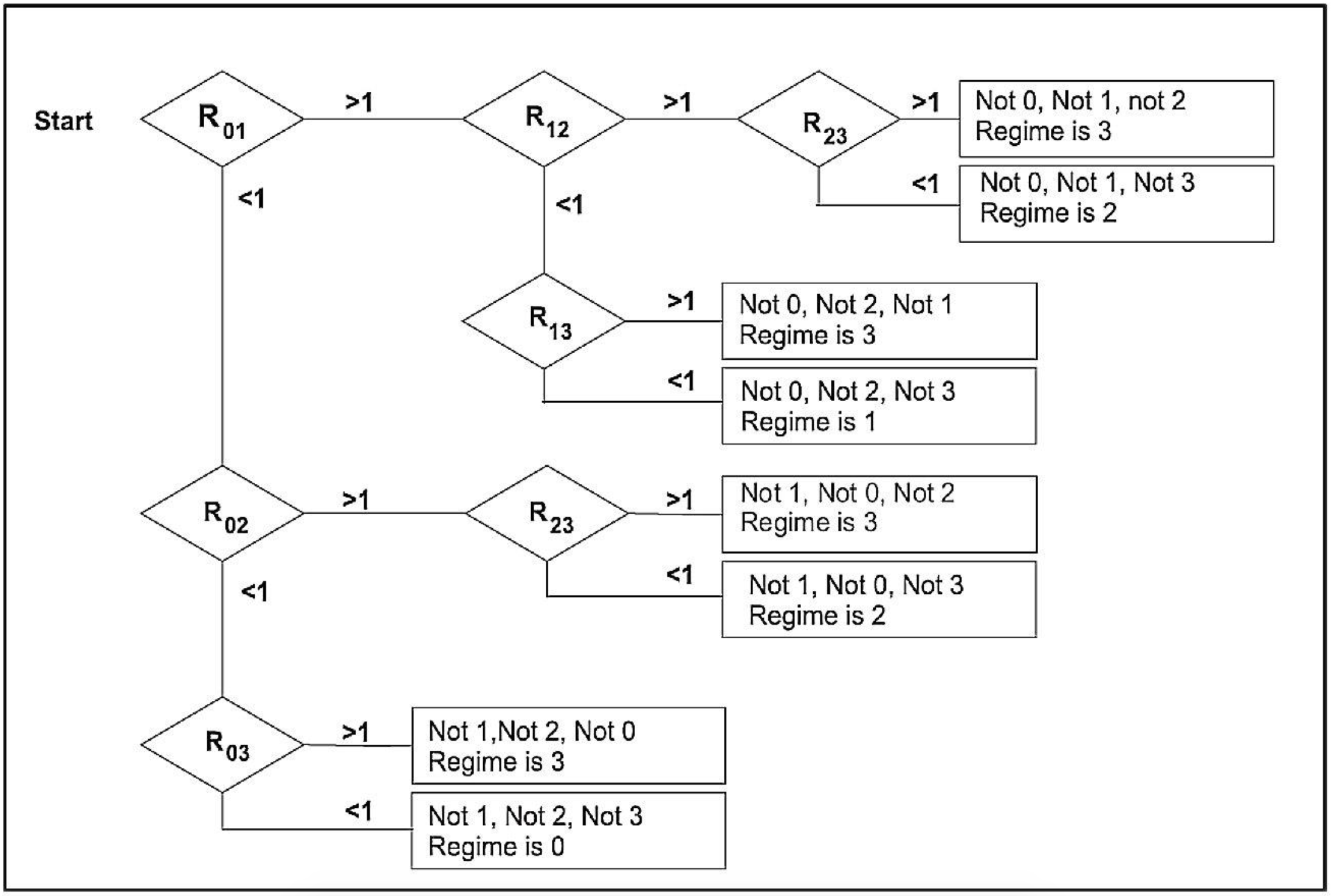
The transition between two flow regimes can be determined by making the two regime equations equal. The resulting Froude number gives the transition line speed. It is however possible that a regime is skipped, so a sliding bed could go to a heterogeneous flow directly, without passing the saltation regime. Figure 6.13-7 shows how to identify the regimes.
The transition Froude numbers are:
The transition fixed bed vs. saltating transport:
\[\ \mathrm{F r}_{\mathrm{0 1}}=\mathrm{4 6 7 9} \cdot \mathrm{C}_{\mathrm{v}}^{\mathrm{1 . 0 8 3}} \cdot \mathrm{f}_{\mathrm{l}}^{\mathrm{1 . 0 6 4}} \cdot \mathrm{C _ { \mathrm { D } }}-\mathrm{0 . 0 6 1 6} \quad\text{with: }\quad \mathrm{R}_{\mathrm{0 1}}=\frac{\mathrm{F r}}{\mathrm{F r}_{\mathrm{0 1}}}\]
The transition fixed bed vs. heterogeneous transport:
\[\ \mathrm{Fr}_{02}=0.1044 \cdot \mathrm{C}_{\mathrm{v}}^{-0.3225} \cdot \mathrm{f}_{\mathrm{l}}^{-1.065} \cdot \mathrm{C}_{\mathrm{D}}^{-0.5906} \quad\text{ with: }\quad \mathrm{R}_{02}=\frac{\mathrm{Fr}}{\mathrm{Fr}_{02}}\]
The transition fixed bed vs. homogeneous transport:
\[\ \mathrm{Fr}_{03}=1.6038 \cdot \mathrm{C}_{\mathrm{v}}^{0.3183} \cdot \mathrm{f}_{\mathrm{l}}^{-0.8837} \cdot \mathrm{C}_{\mathrm{D}}^{-0.7496} \quad\text{ with: }\quad \mathrm{R}_{03}=\frac{\mathrm{Fr}}{\mathrm{Fr}_{03}}\]
The transition saltating transport vs. heterogeneous transport:
\[\ \mathrm{F r}_{12}=\mathrm{6 . 8 3 5 9} \cdot \mathrm{C}_{\mathrm{v}}^{\mathrm{0 . 2 2 6 3}} \cdot \mathrm{f}_{\mathrm{l}}^{-\mathrm{0 . 2 3 3 4}} \cdot \mathrm{C _ { 0 }}^{-\mathrm{0 . 3 8 4 0}} \quad\text{ with: }\quad \mathrm{R}_{12}=\frac{\mathrm{F r}}{\mathrm{F r}_{\mathrm{1 2}}}\]
The transition saltating transport vs. homogeneous transport:
\[\ \mathrm{Fr}_{13}=12.522 \cdot \mathrm{C}_{\mathrm{v}}^{0.5153} \cdot \mathrm{f}_{\mathrm{l}}^{-0.3820} \cdot \mathrm{C}_{\mathrm{D}}-0.5724 \quad\text{ with: }\quad \mathrm{R}_{13}=\frac{\mathrm{Fr}}{\mathrm{Fr}_{13}}\]
The transition heterogeneous transport vs. homogeneous transport:
\[\ \mathrm{Fr}_{23}=40.38 \cdot \mathrm{C}_{\mathrm{v}}^{1.075} \cdot \mathrm{f}_{1}^{-0.6700} \cdot \mathrm{C}_{\mathrm{D}}-0.9375 \quad\text{ with: }\quad \mathrm{R}_{23}=\frac{\mathrm{Fr}}{\mathrm{Fr}_{23}}\]
6.13.6 Conclusions & Discussion
Turian & Yuan (1977) developed a set of 4 empirical equations for 4 flow regimes based on a large set of public available experiments and a set of experiments carried out by themselves. Based on these 4 equations a set of 6 possible transition equations were derived. The 4 flow regimes, stationary bed, saltation, heterogeneous transport and homogeneous transport do not cover all possible flow regimes. The sliding bed regime and the sheet flow regime are not covered independently. Often it is very hard to distinguish between the flow regimes based on visual observations, so it is very well possible that in the transition regions the wrong regime has been chosen. Turian & Yuan (1977) choose for a fixed form of their equations.
\[\ \mathrm{f_{m}-f_{l}=\frac{\lambda_{m}}{4}-\frac{\lambda_{l}}{4}=K \cdot C_{v}^{\alpha} \cdot f_{1}^{\beta} \cdot\left(\frac{4}{3} \cdot \frac{R_{s d} \cdot g \cdot d}{v_{t}^{2}}\right)^{\gamma} \cdot\left(\frac{v_{l s}^{2}}{R_{s d} \cdot g \cdot D_{p}}\right)^{\delta}}\]
Basically all 4 equations have one term for the solids effect and one term for the Darcy Weisbach pressure losses in clean water. This limits the physical meaning of the equations. It is very well possible that the real physics justify 2 or more terms. The fact that Turian & Yuan (1977) use the Froude number and the drag coefficient, implies that the relation between pipe diameter Dp and line speed vls is fixed and the relation between particle diameter d and terminal settling velocity vt is fixed. A combination of, for example, the particle diameter d and the thickness of the viscous sub-layer δ, is not possible this way, leaving out other possible physical phenomena.
The difference between spatial and transport concentration is only important for the stationary bed regime, for the other regimes the difference between the two concentrations is negligible and much smaller than the scatter. The stationary bed equation most probably uses the constant transport concentration.
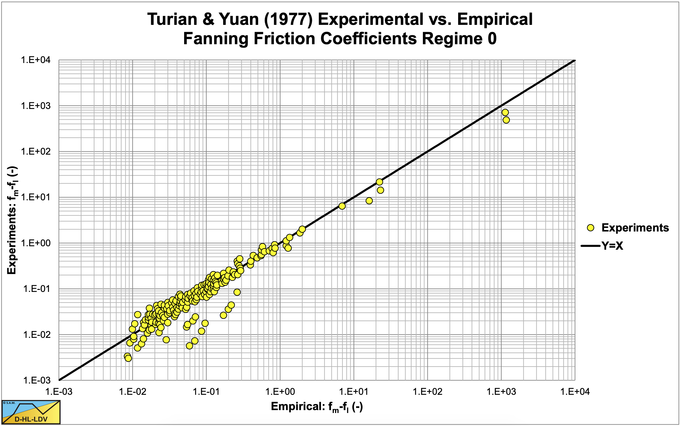
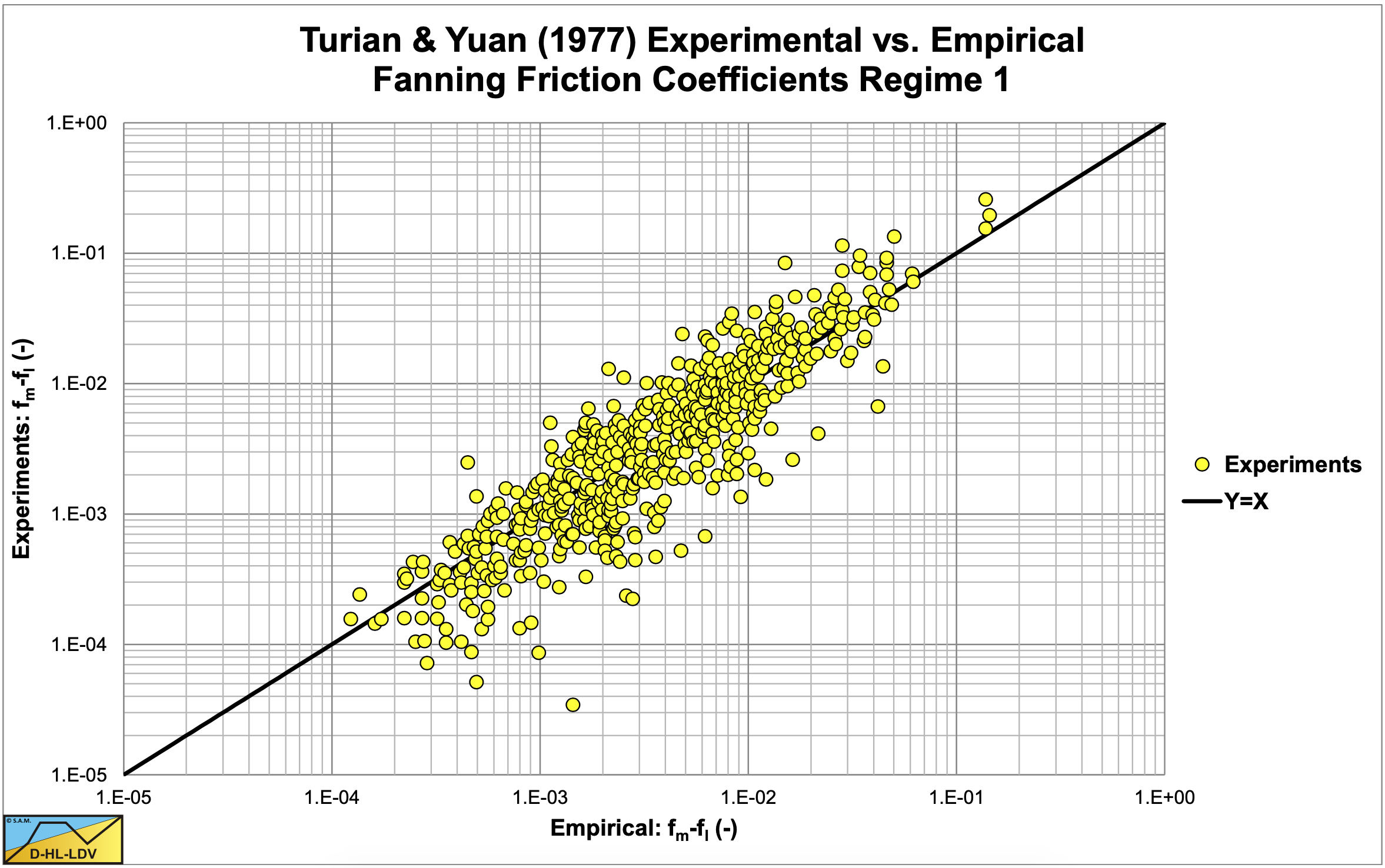
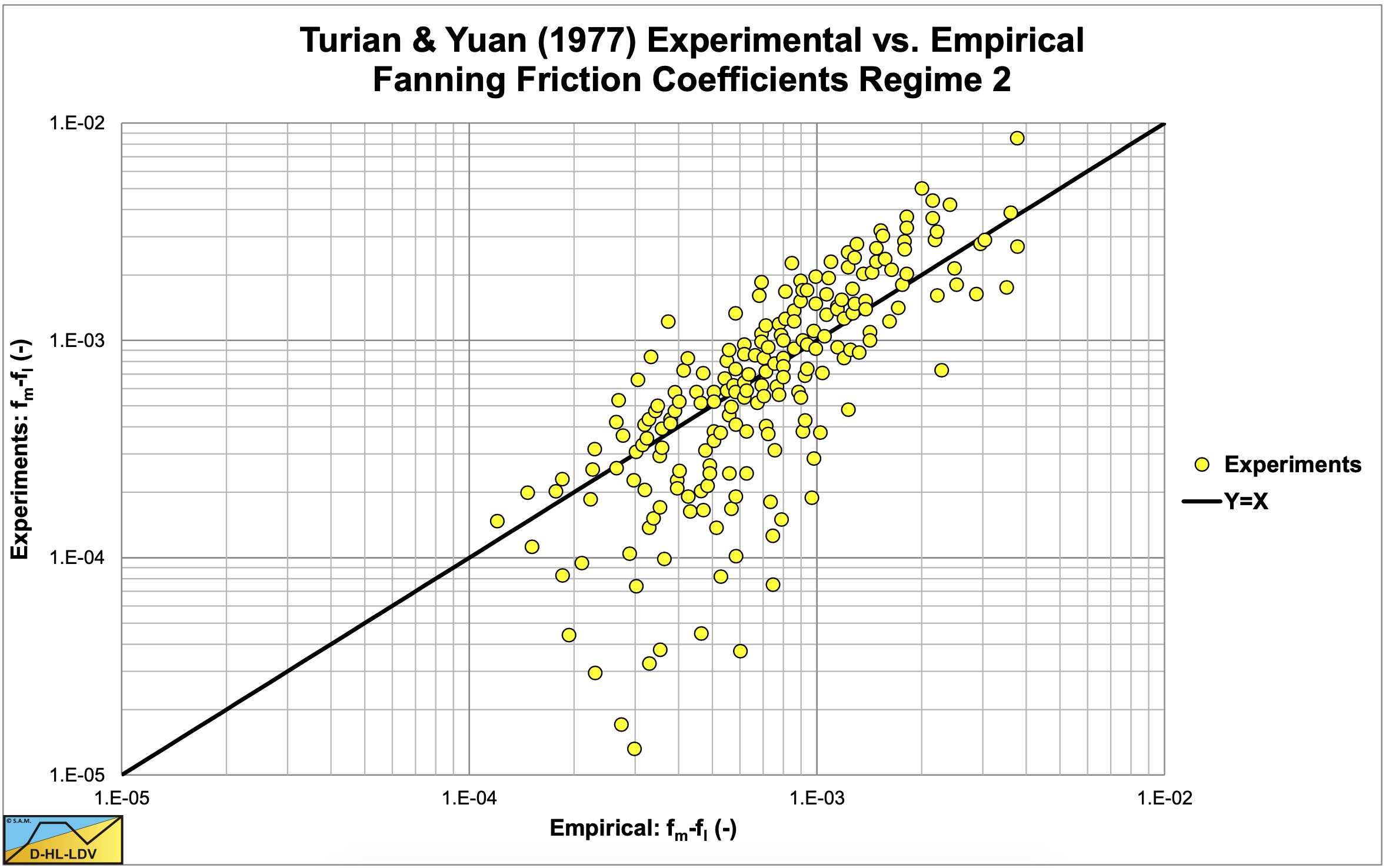
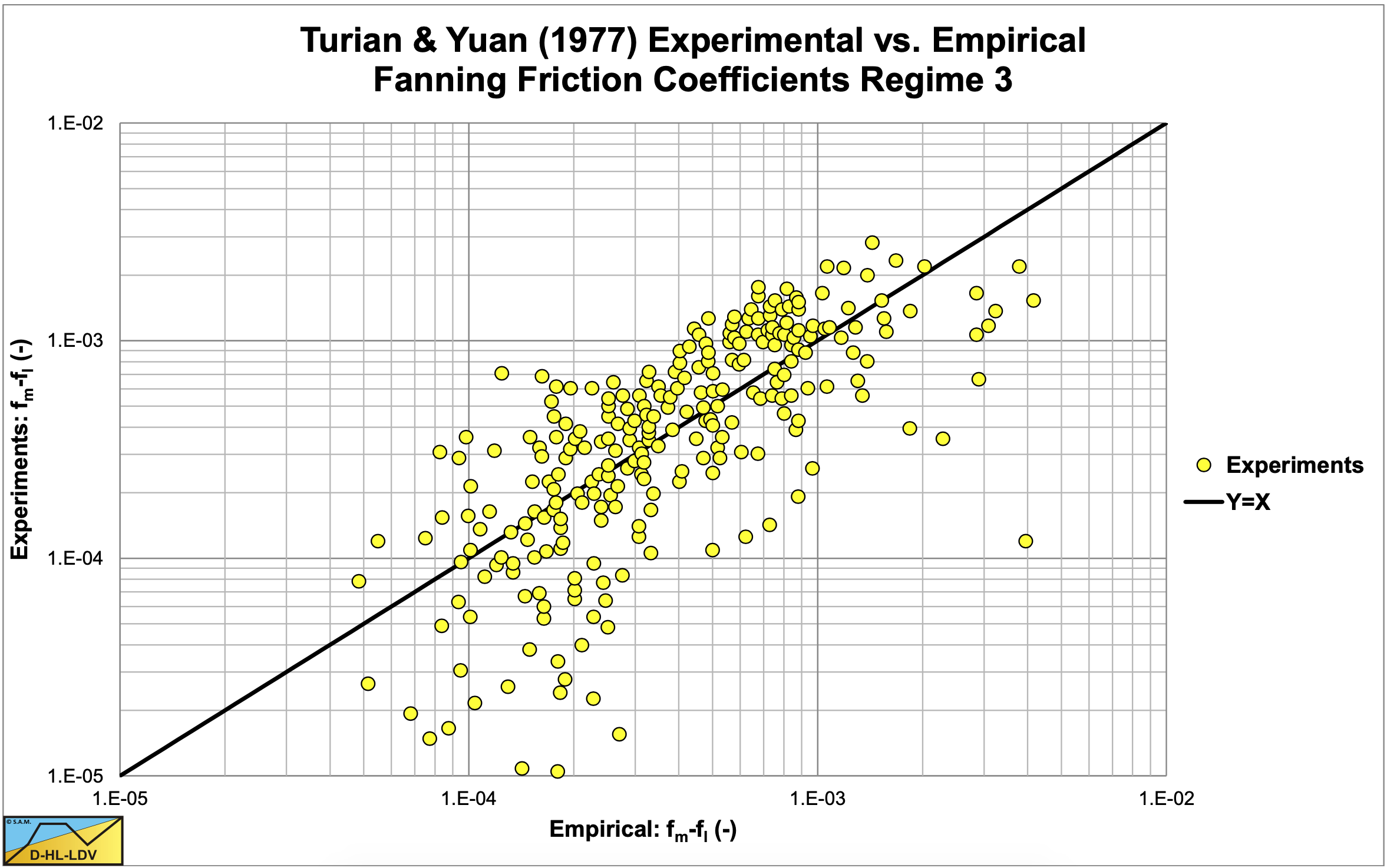
The correlations of the experiments with the empirical equations are shown in Figure 6.13-1, Figure 6.13-2, Figure 6.13-3 and Figure 6.13-4. These graphs show quit some scatter. Most of the experiments were carried out in sand with pipe diameters between 0. 508 m and 0.1524 m (2 and 6 inch). This implies that the resulting equations most probably have value for these conditions.
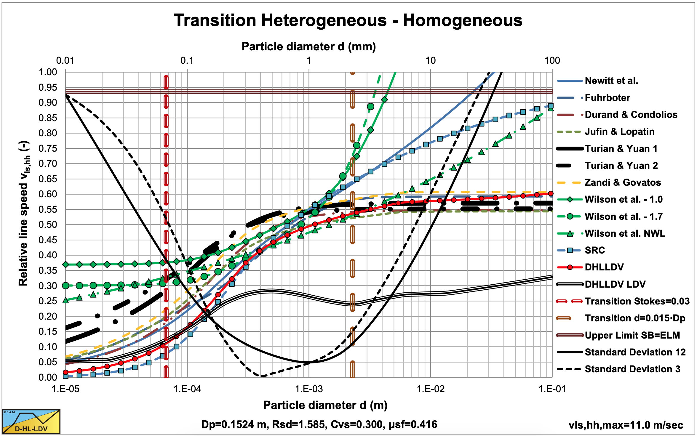
A comparison of the transition line speed of the heterogeneous and homogeneous regimes, with other models, Figure 6.13-8, shows that the equations give a reasonable prediction for larger particles (d>0.3 mm) at higher concentrations, based on the saltation regime 1 and the heterogeneous regime 2. For very small particles, the saltation and heterogeneous equations overestimate the pressure losses. The velocity on the vertical axis has been made relative by dividing by the line speed in the lower right corner.
Analyzing the 4 flow regimes of Turian & Yuan (1977) and comparing them with other models results in a sort of conversion table.
|
Turian & Yuan (1977) |
Others, Miedema (2013S) |
|
Regime 0: Stationary bed. |
Stationary bed and sliding bed. |
|
Regime 1: Saltation. |
Heterogeneous transport and sheet flow or Fixed/sliding bed (thin layer) with heterogeneous transport above the bed. |
|
Regime 2: Heterogeneous transport. |
Heterogeneous transport above the Limit Deposit Velocity and pseudo homogeneous transport. |
|
Regime 3: Homogeneous transport. |
Pseudo homogeneous and homogeneous transport. |