6.9: A.D. Thomas (1976) and (1979)

6.12.1 Head Losses

A.D. Thomas (1976) investigated scale-up methods for pipeline transport of slurries. To do so he investigated pipes with diameters ranging from 50 mm to 300 mm diameter. The main purpose of this research was to find relations between the excess hydraulic gradient (the solids effect) and the pipe diameter and the line speed. To do so, particles are divided (based on the particle diameter) into 3 flow regimes. Very fine particles are supposed to behave according to the Equivalent Liquid Model (ELM), with or without a correction for the viscosity. Coarse particles are supposed to behave according to heterogeneous models, for which the Durand & Condolios (1952) model was chosen. Medium sized particles behave according to a pseudo heterogeneous flow regime, which is an intermediate between the homogeneous regime and the heterogeneous regime. In all cases this is considered for normal operational line speeds. The hydraulic gradient for pure liquid flow is defined as:

\[\ \mathrm{i}_{\mathrm{l}}=\frac{\lambda_{\mathrm{l}} \cdot \mathrm{v}_{\mathrm{l s}}^{2}}{2 \cdot \mathrm{g} \cdot \mathrm{D}_{\mathrm{p}}}\]

For rough pipes it is assumed that the Darcy Weisbach friction factor is reversely proportional to the Reynolds number to the power of 0.2. This power depends on the Reynolds number and also on the roughness of the pipe wall. Using this assumption gives for the hydraulic gradient:

\[\ \mathrm{i}_{\mathrm{l}}=\frac{\lambda_{\mathrm{l}} \cdot \mathrm{v}_{\mathrm{l s}}^{2}}{2 \cdot \mathrm{g} \cdot \mathrm{D}_{\mathrm{p}}}=\mathrm{A} \cdot \mathrm{v}_{\mathrm{l} \mathrm{s}}^{\mathrm{1 . 8}} \cdot \mathrm{D}_{\mathrm{p}}^{-\mathrm{1 . 2}}\]

Thomas (1976) found from his experiments:

\[\ \mathrm{i}_{\mathrm{l}}=\mathrm{A} \cdot \mathrm{v}_{\mathrm{l} \mathrm{s}}^{\mathrm{1 . 7 7}} \cdot \mathrm{D}_{\mathrm{p}}^{-\mathrm{1 . 1 8}}\]

Which is close to the theoretical proportionalities. For the ELM the following relation was chosen:

\[\ \mathrm{i}_{\mathrm{m}}=\mathrm{A} \cdot \mathrm{v}_{\mathrm{l} \mathrm{s}}^{\mathrm{1 . 7 7}} \cdot \mathrm{D}_{\mathrm{p}}^{-\mathrm{1 . 1 8}} \cdot \frac{\rho_{\mathrm{m}}}{\rho_{\mathrm{l}}}\]

Now suppose the Durand & Condolios (1952) equation is used for the heterogeneous regime, this would give the following proportionalities:

\[\ \mathrm{i}_{\mathrm{m}}-\mathrm{i}_{\mathrm{l}}=\mathrm{K}_{\mathrm{1}} \cdot \mathrm{v}_{\mathrm{l} \mathrm{s}}^{-\mathrm{3}} \cdot \mathrm{D}_{\mathrm{p}}^{\mathrm{1 . 5}} \cdot \mathrm{i}_{\mathrm{l}} \cdot \mathrm{C}_{\mathrm{v} \mathrm{t}}\]

Substituting the equation for the pure liquid hydraulic gradient gives:

\[\ \mathrm{i}_{\mathrm{m}}-\mathrm{i}_{\mathrm{l}}=\mathrm{K}_{\mathrm{1}} \cdot \mathrm{v}_{\mathrm{l} \mathrm{s}}^{-\mathrm{3}} \cdot \mathrm{D}_{\mathrm{p}}^{\mathrm{1 . 5}} \cdot \mathrm{i}_{\mathrm{l}} \cdot \mathrm{A} \cdot \mathrm{v}_{\mathrm{l} \mathrm{s}}^{\mathrm{1} \mathrm{8}} \cdot \mathrm{D}_{\mathrm{p}}^{-\mathrm{1 . 2}} \cdot \mathrm{C}_{\mathrm{v t}}=\mathrm{K}_{2} \cdot \mathrm{v}_{\mathrm{l} \mathrm{s}}^{-\mathrm{1 . 2}} \cdot \mathrm{D}_{\mathrm{p}}^{\mathrm{0 . 3}} \cdot \mathrm{C}_{\mathrm{v t}}\]

So the excess hydraulic gradient is proportional to the line speed to a power of -1.2 and proportional to the pipe diameter to a power of 0.3. This behavior is generally accepted to describe the heterogeneous behavior of coarse particles. Whether the linear proportionality of the delivered concentration holds is a question. Charles (1970) found that this is the case in the sliding bed regime, but not always in the heterogeneous regime, especially at high concentrations.

It was found that the proportionality with the line speed to a power of -1.2 correlated well with the experimental data up to a certain line speed, after which the power became positive. This certain line speed in fact is the transition (intersection point) between the heterogeneous and the homogeneous regime. The approach of Zandi & Govatos (1967), using two equations, was rejected, because the powers found did not match the experimental data. The Durand & Condolios (1952) approach gives good results for small line speeds, but not for high line speeds, since this approach gives a solids effect that asymptotically reaches zero for high line speeds, while experiments have shown that the asymptotic value should match the ELM behavior. The method of Charles (1970) solves these problems and gives an equation with the following proportionalities:

\[\ \begin{aligned} \mathrm{i}_{\mathrm{m}}-\mathrm{i}_{\mathrm{l}}=\mathrm{K}_{\mathrm{3}} \cdot \mathrm{v}_{\mathrm{l} \mathrm{s}}^{-\mathrm{1 . 2}} \cdot \mathrm{D}_{\mathrm{p}}^{\mathrm{0 . 3}} \cdot \mathrm{C}_{\mathrm{v t}}+\mathrm{K}_{4} \cdot \mathrm{v}_{\mathrm{l} \mathrm{s}}^{\mathrm{1 . 8}} \cdot \mathrm{D}_{\mathrm{p}}^{-\mathrm{1 . 2}} \cdot \mathrm{R}_{\mathrm{s d}} \cdot \mathrm{C}_{\mathrm{v t}}\\
\text{Durand & Condolios}\quad \quad\quad\text{ELM}\quad\quad\quad\quad\quad \end{aligned}\]

This equation will do well for very small line speeds if the second term is negligible and for very large line speeds when the first term is negligible, but it will give too high values in between and this is the region we are interested in for pseudo heterogeneous flow. Multiplying the second term with a factor 0.7 gives a good match with the experiments of Thomas (1976), giving:

\[\ \mathrm{i}_{\mathrm{m}}-\mathrm{i}_{\mathrm{l}}=\mathrm{K}_{\mathrm{3}} \cdot \mathrm{v}_{\mathrm{l} \mathrm{s}}^{-\mathrm{1 . 2}} \cdot \mathrm{D}_{\mathrm{p}}^{\mathrm{0 . 3}} \cdot \mathrm{C}_{\mathrm{v t}}+\mathrm{0 . 7} \cdot \mathrm{K}_{4} \cdot \mathrm{v}_{\mathrm{l} \mathrm{s}}^{\mathrm{1} .8} \cdot \mathrm{D}_{\mathrm{p}}^{-\mathrm{1 . 2}} \cdot \mathrm{R}_{\mathrm{s d}} \cdot \mathrm{C}_{\mathrm{v t}}\]

This solves the proportionalities of the excess hydraulic gradient with the line speed. However this does not solve the power of the pipe diameter in the first term. The positive power does not correlate the data for different pipe diameters for medium sands. This would require a negative power.

Vocadlo & Charles (1972) proposed the following equation for the transition of the heterogeneous to the homogeneous regime:

\[\ \mathrm{i}_{\mathrm{m}}=\mathrm{K}_{5} \cdot \mathrm{C}_{\mathrm{v} \mathrm{t}} \cdot \mathrm{R}_{\mathrm{sd}} \cdot \frac{\mathrm{v}_{\mathrm{t}}}{\mathrm{v}_{\mathrm{l s}}}+\mathrm{i}_{\mathrm{l}} \cdot\left(\frac{\mathrm{\mu}_{\mathrm{m}}}{\mu_{\mathrm{l}}}\right) \cdot\left(\mathrm{1}+\mathrm{R}_{\mathrm{s d}} \cdot \mathrm{C}_{\mathrm{v t}}\right)^{0.8}\]

The first term, the heterogeneous solids effect, is very similar to the Newitt et al. (1955) equation for heterogeneous transport. The second term is not proportional with the volumetric concentration and follows the same trend as the Talmon (2011) model for homogeneous transport, based on a particle free viscous sub-layer. The second term also follows the model of Jufin & Lopatin (1966), based on experiments in the pseudo heterogeneous and homogeneous regimes. The second term also adjusts for the apparent viscosity due to the solids in the liquid. This equation can be simplified to:

\[\ \mathrm{i}_{\mathrm{m}}-\mathrm{i}_{\mathrm{l}}=\mathrm{K}_{\mathrm{6}} \cdot \mathrm{v}_{\mathrm{l} \mathrm{s}}^{-\mathrm{1}}+\mathrm{K}_{7} \cdot \mathrm{v}_{\mathrm{l} \mathrm{s}}^{\mathrm{1} .8} \cdot \mathrm{D}_{\mathrm{p}}^{-\mathrm{1 . 2}}\]

Now the excess hydraulic gradient in the first term does not depend on the pipe diameter anymore. For an intermediate particle size of d=0.48 mm Thomas (1976) found that this is close, however for the smaller particle size of d=0.18 mm he found that the power of the pipe diameter in the first term should be negative to explain for the trends in the experimental data. He proposes the following equation:

\[\ \begin{array}{left}\mathrm{i}_{\mathrm{m}}-\mathrm{i}_{\mathrm{l}}=\mathrm{K}_{\mathrm{8}} \cdot \mathrm{v}_{\mathrm{l} \mathrm{s}}^{-\mathrm{1 . 2}} \cdot \mathrm{D}_{\mathrm{p}}^{\mathrm{b}}+\mathrm{K}_{\mathrm{9}} \cdot \mathrm{v}_{\mathrm{l} \mathrm{s}}^{\mathrm{1 . 8}} \cdot \mathrm{D}_{\mathrm{p}}^{-\mathrm{1 . 2}}\\
\mathrm{o} \mathrm{r}\\
\mathrm{i}_{\mathrm{m}}=\mathrm{K}_{\mathrm{8}} \cdot \mathrm{v}_{\mathrm{l} \mathrm{s}}^{-\mathrm{1 . 2}} \cdot \mathrm{D}_{\mathrm{p}}^{\mathrm{b}}+\mathrm{K}_{\mathrm{1 0}} \cdot \mathrm{v}_{\mathrm{l} \mathrm{s}}^{\mathrm{1} \cdot \mathrm{8}} \cdot \mathrm{D}_{\mathrm{p}}^{-\mathrm{1 . 2}}\end{array}\]

The first term now contains the power b for the pipe diameter, which is positive for coarse particles, close to zero for intermediate particles and negative for fine particles.

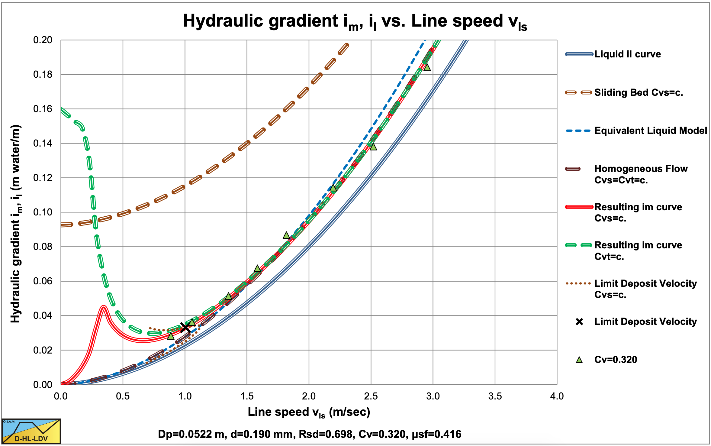
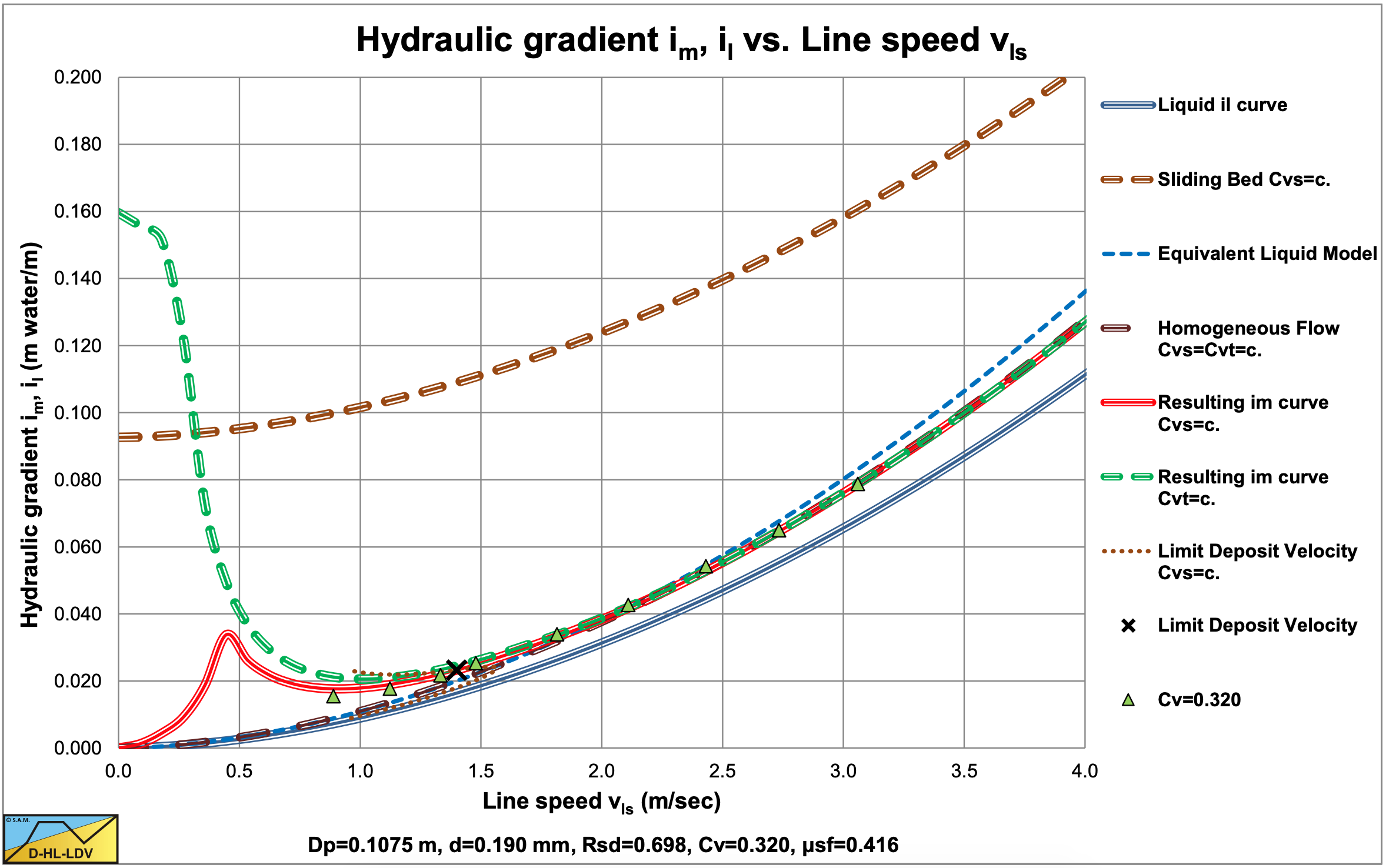
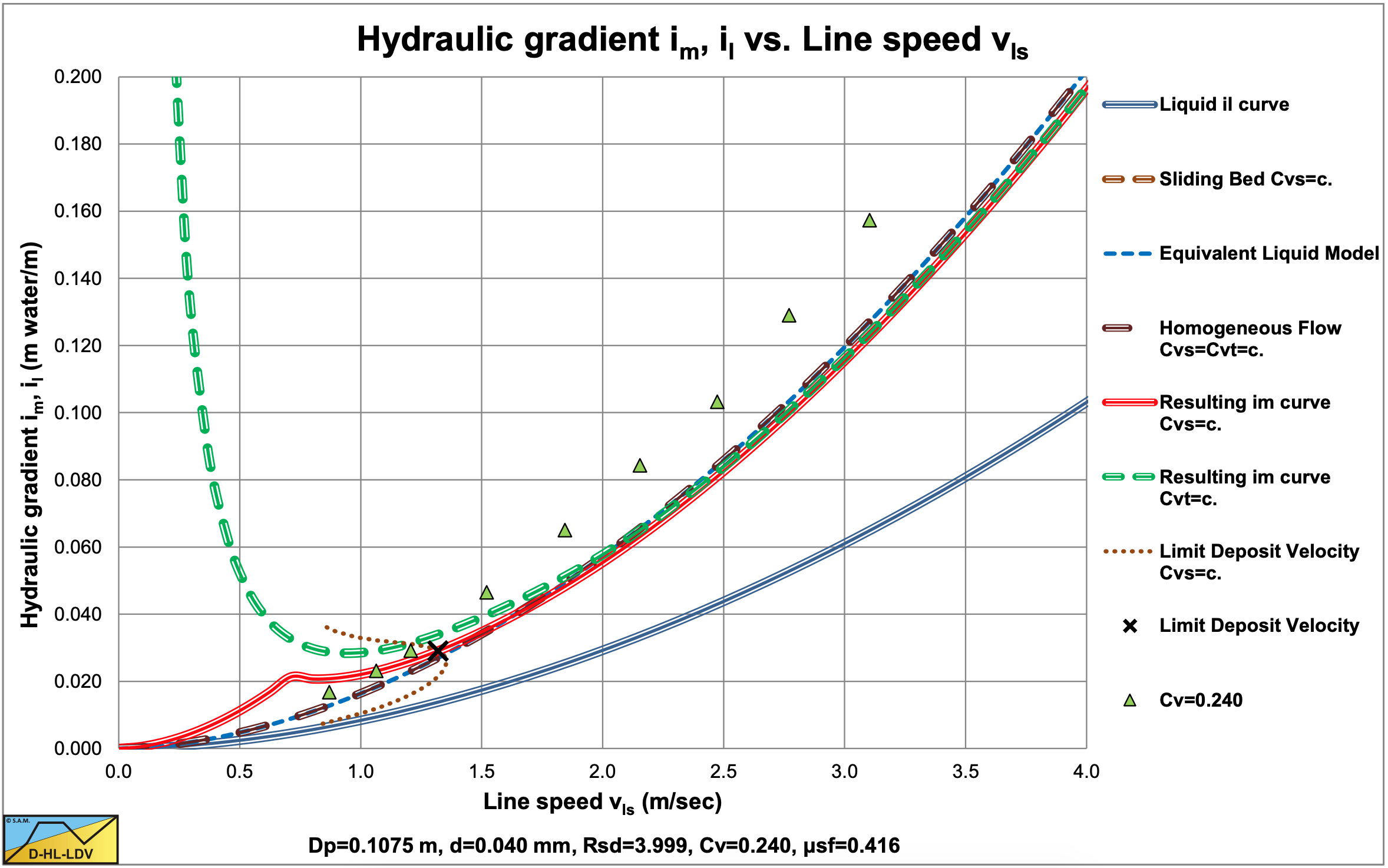
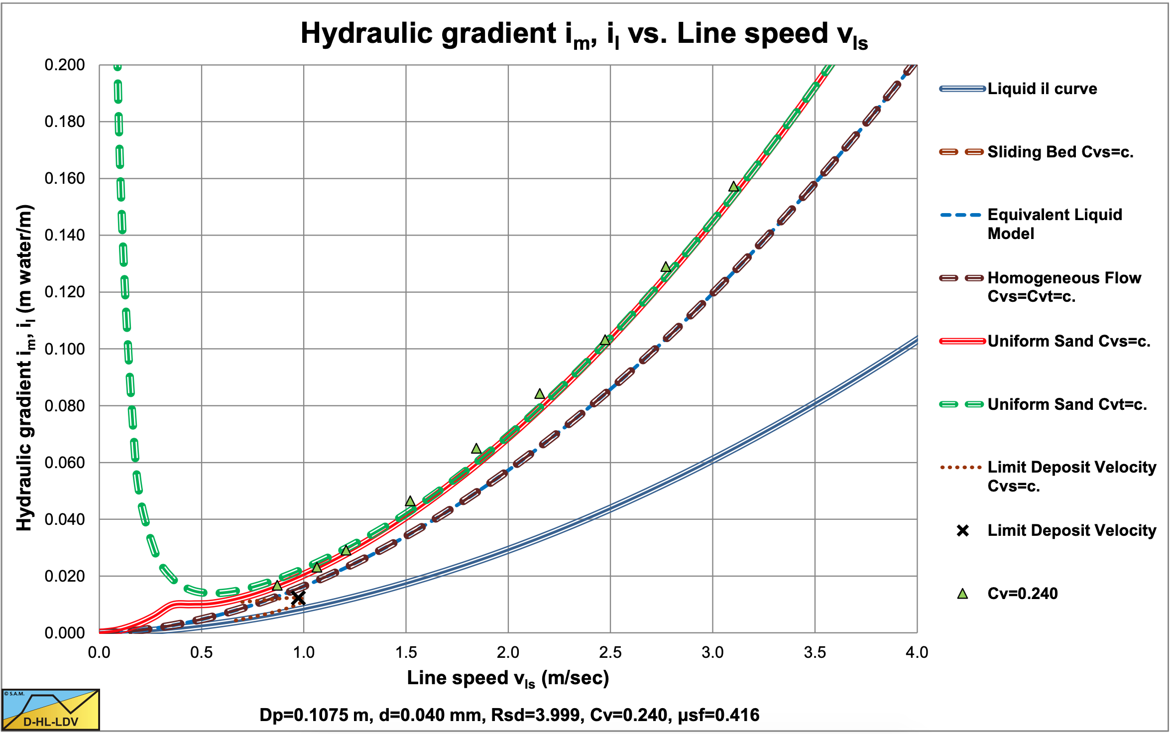
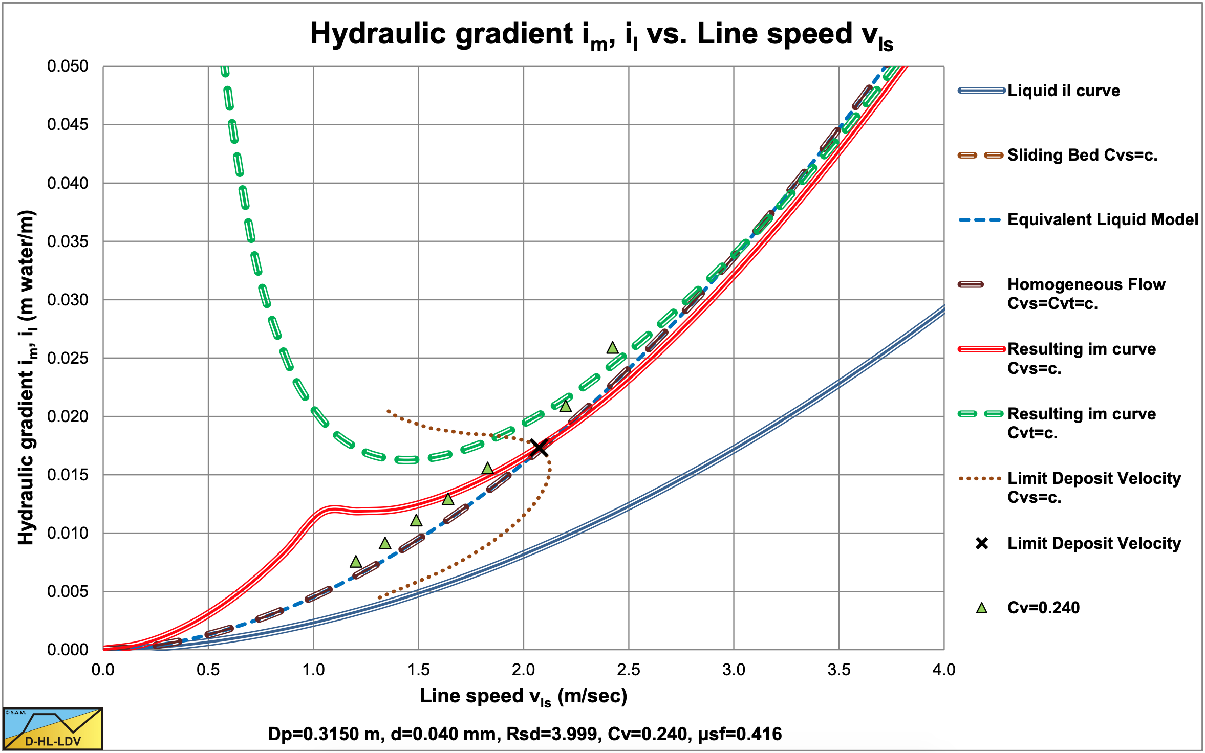
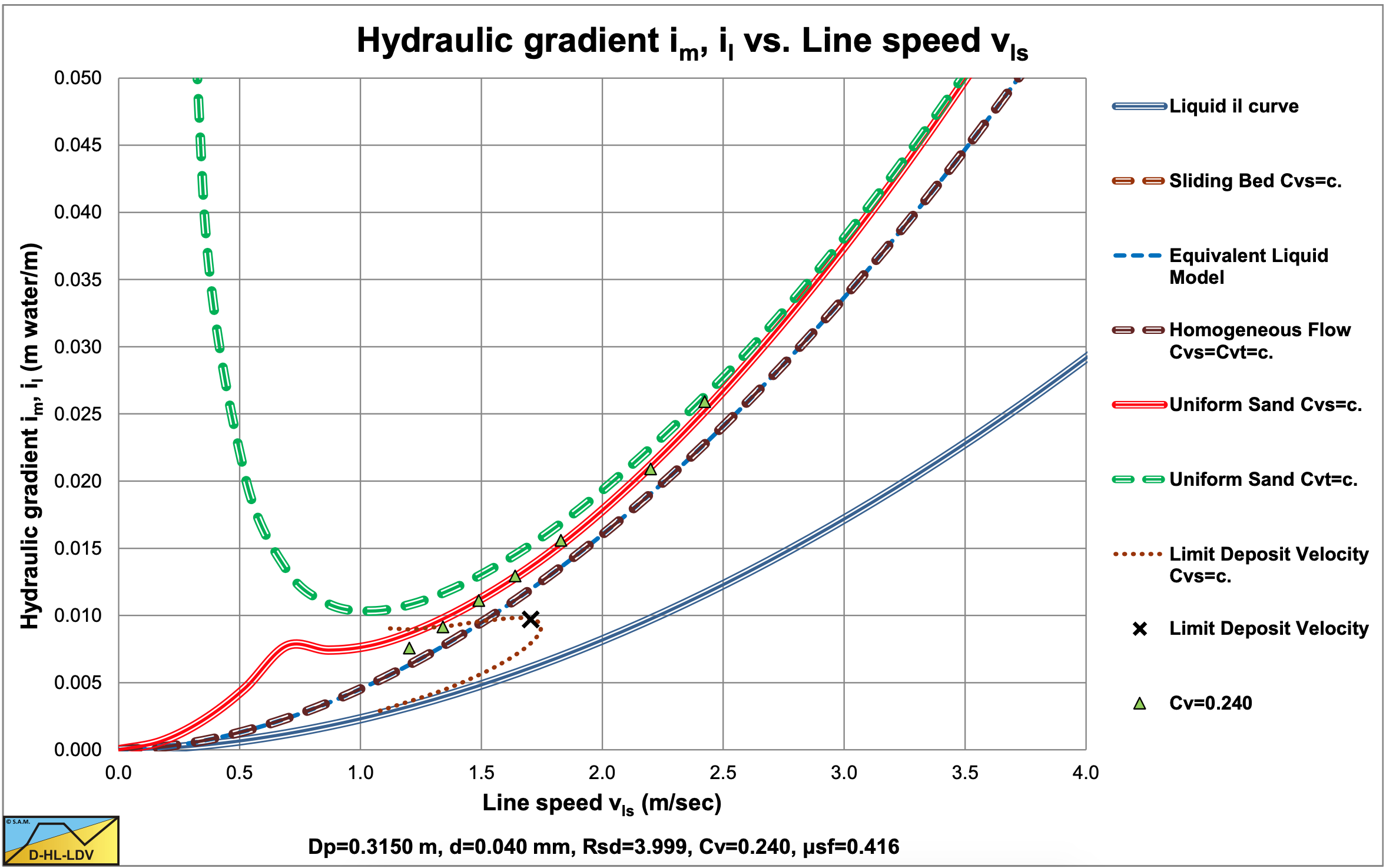
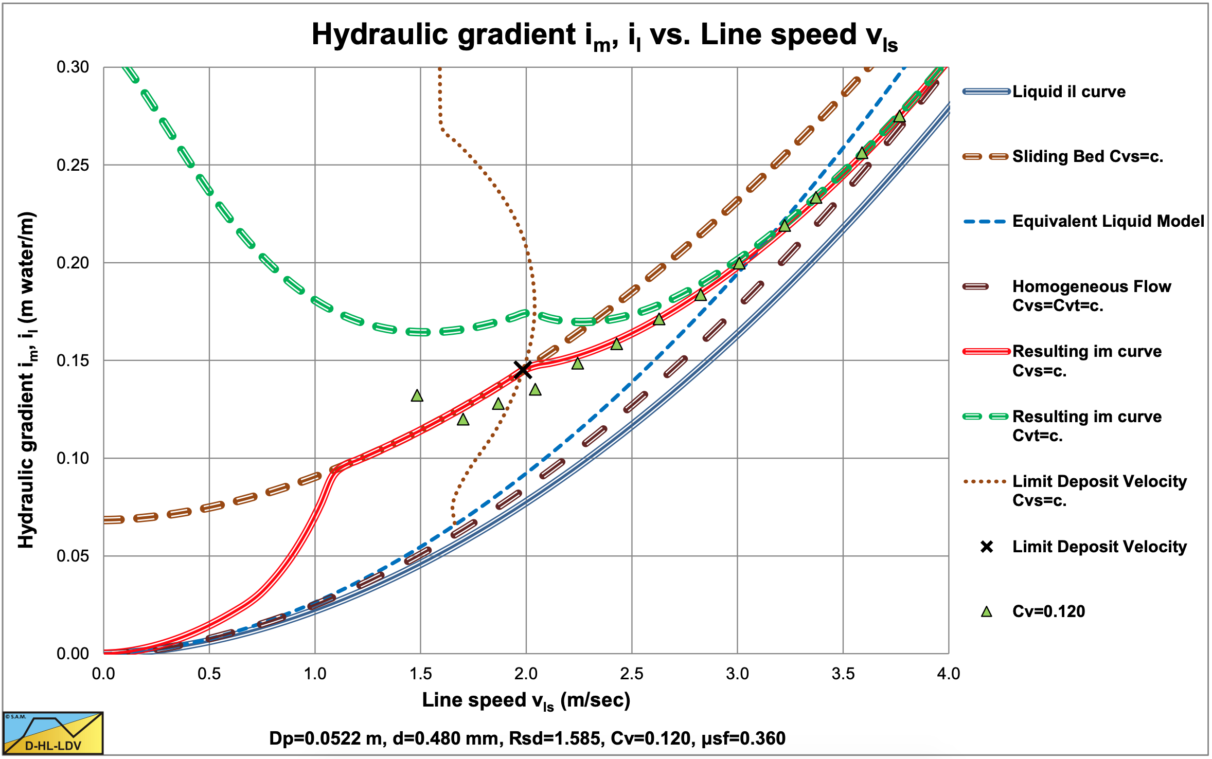
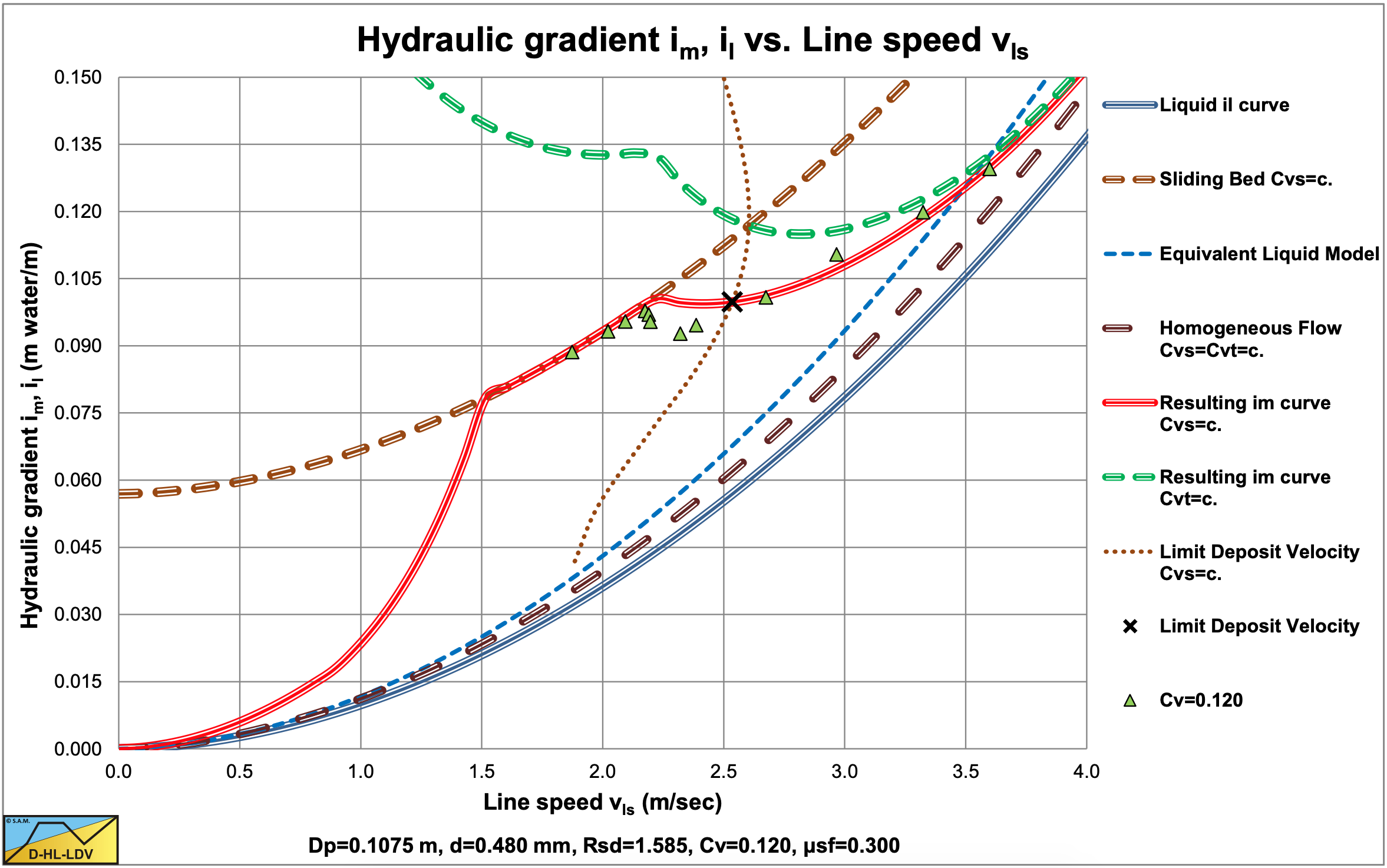
Figure 6.12-1, Figure 6.12-2, Figure 6.12-3 and Figure 6.12-5 show that fine particles at relatively high line speeds result in homogeneous behavior according to the ELM. The graphs for coal slurry are according to the ELM without correction for the viscosity and the slurry density. The graphs for iron ore include a correction for the viscosity and the slurry density.

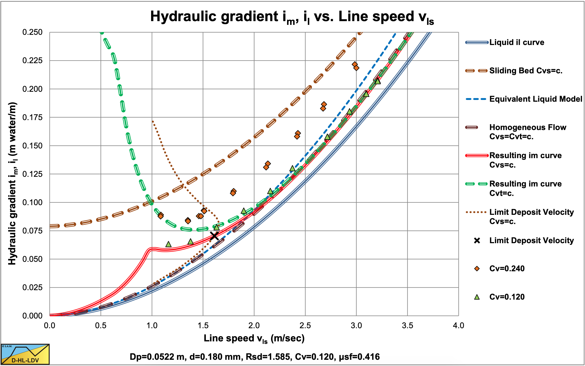
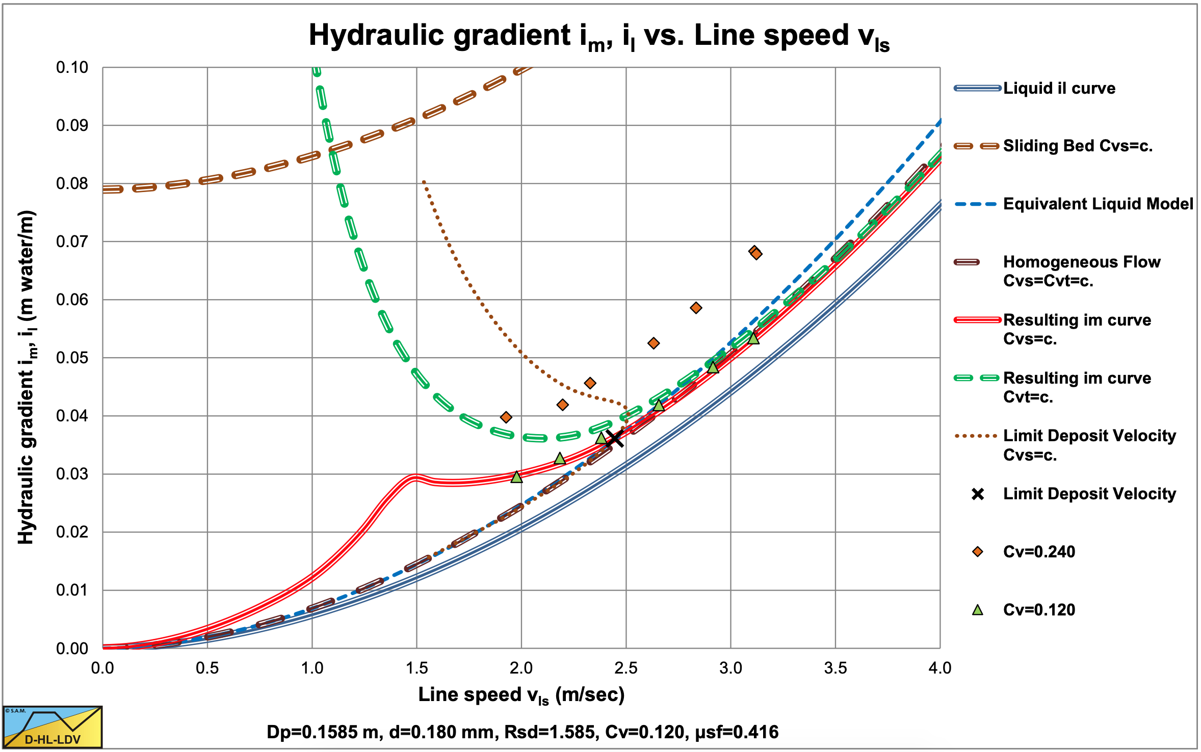
Figure 6.12-7, Figure 6.12-8, Figure 6.12-9 and Figure 6.12-10 show some data for the d=0.18 mm sand and the d=0.48 mm sand in different pipe diameters, compared with the DHLLDV Framework. The DHLLDV Framework uses a power of about 0-0.15 for the pipe diameter in the first term of the equations, the power b. Still the results of DHLLDV match well with the experimental data of Thomas (1976). How can this be explained?

Thomas (1976) assumes a power of -1.2 for the line speed in the first term of the above equation. When the pipe diameter increases however, also the line speed of the experiments increases, since most experiments are carried out above the LDV. In the pseudo heterogeneous region, the excess hydraulic gradient curves flatten, so the power of -1.2 of the line speed in the first term may be too high, a more negative power is required. Now suppose the power is a and the LDV increases with the square root of the pipe diameter. This gives the following equation:

\[\ \begin{array}{left} \mathrm{v}_{\mathrm{l} \mathrm{s}, \mathrm{ld} \mathrm{v}} \propto \mathrm{D}_{\mathrm{p}}^{\mathrm{1 / 2}}\text{ and }\mathrm{D}_{\mathrm{p}} \propto \mathrm{v}_{\mathrm{l} \mathrm{s}, \mathrm{l d v}}^{\mathrm{2}}\\
\mathrm{i}_{\mathrm{m}, \mathrm{l d v}} \propto \mathrm{v}_{\mathrm{l} \mathrm{s}, \mathrm{ld v}}^{\mathrm{a}} \cdot \mathrm{D}_{\mathrm{p}}^{\mathrm{b}} \propto \mathrm{v}_{\mathrm{l} \mathrm{s}, \mathrm{ld} \mathrm{v}}^{\mathrm{a}} \cdot \mathrm{v}_{\mathrm{l} \mathrm{s}, \mathrm{l d v}}^{\mathrm{b} / 2}=\mathrm{v}_{\mathrm{l s}, \mathrm{ld v}}^{\mathrm{a}+\mathrm{b} / \mathrm{2}}\end{array}\]

Figure 6.12-1: The hydraulic gradient of a coal slurry, d=0.19 mm, in an 0.0522 m diameter pipe.

Figure 6.12-2: The hydraulic gradient of a coal slurry, d=0.19 mm, in an 0.1075 m diameter pipe.

Suppose in reality the power a=-1.7 and the power b=0, so a+b/2=-1.7 or a=-1.7-b/2 or b=2·(-1.7-a). Using a power of -1.2 would give a power b=-1. The Wilson et al. (2006) model uses a=-1.7 for uniform sands. Zandi & Govatos (1967) use a=-1.86 and the DHLLDV Framework a=-1.7, also for uniform sands. The conclusion is, that different values for the power a result in different values for the power b. The conclusion of Thomas (1976) regarding the power of the pipe diameter should be interpreted with care.

Figure 6.12-3: The hydraulic gradient of an iron ore slurry, d=0.04 mm, in an 0.1075 m diameter pipe, without Thomas (1965) viscosity.

Figure 6.12-4: The hydraulic gradient of an iron ore slurry, d=0.04 mm, in an 0.1075 m diameter pipe, including Thomas (1965) viscosity.

Figure 6.12-5: The hydraulic gradient of an iron ore slurry, d=0.04 mm, in an 0.3150 m diameter pipe, without Thomas (1965) viscosity.

Figure 6.12-6: The hydraulic gradient of an iron ore slurry, d=0.04 mm, in an 0.3150 m diameter pipe, including Thomas (1965) viscosity.

Figure 6.12-7: The hydraulic gradient of a sand slurry, d=0.18 mm, in an 0.0522 m diameter pipe.

Figure 6.12-8: The hydraulic gradient of a sand slurry, d=0.18 mm, in an 0.1585 m diameter pipe.

Figure 6.12-9: The hydraulic gradient of a sand slurry, d=0.48 mm, in an 0.0522 m diameter pipe.

Figure 6.12-10: The hydraulic gradient of a sand slurry, d=0.48 mm, in an 0.1075 m diameter pipe.

6.12.2 The Limit Deposit Velocity

Based on the experiments of Thomas (1976) with d=0.18 mm sand at volumetric concentrations of 12% and 24%, the following equation was found for the Durand Froude number F_L:

\[\ \mathrm{F_{L}=\frac{v_{l s, ld v}}{\sqrt{2 \cdot g \cdot R_{s d} \cdot D_{p}}}=0.81 \cdot D_{p}^{-0.137}}\]

The derivation is based on the experimental data of Thomas (1976) and may not be very accurate. The main conclusion from this exercise is that the Durand Froude number decreases with increasing pipe diameter, which was also found by Jufin & Lopatin (1966). According to Durand & Condolios (1952) and Gibert (1960) the Durand Froude number F_L is independent from the pipe diameter. Jufin & Lopatin (1966) found a power of -0.167 and here a power of -0.137 was found. This is for fine to coarse particles, but probably not for very fine particles and very coarse particles. Thomas (1979) found that the relation between the LDV and the pipe diameter for fine to coarse particles has a dependency with a power between 0.1 as a lower limit and 0.5 as an upper limit.

Thomas (1979) derived an equation for very small particles, proving that there is a lower limit to the LDV or LSDV. The method is based on the fact that particles smaller than the thickness of the viscous sub layer will be in suspension due to turbulent eddies in the turbulent layer, but may still settle in the laminar viscous sub layer.

The thickness of the thin layer is assumed to be equal to the thickness of the viscous sub layer:

\[\ \delta_{\mathrm{v}}=\mathrm{5} \cdot \frac{v_{\mathrm{l}}}{\mathrm{u}_{*}}\]

By using a force balance on a very thin bed layer in the viscous sub layer, he found the following equation, using a factor 5 for the thickness of the viscous sub-layer instead of the factor 11.6:

\[\ \mathrm{v}_{\mathrm{l s}, \mathrm{ld v}}=\mathrm{1 . 4 9} \cdot\left(\mathrm{g} \cdot \mathrm{R}_{\mathrm{s d}} \cdot \mathrm{C}_{\mathrm{v b}} \cdot v_{\mathrm{l}} \cdot \mathrm{\mu}_{\mathrm{s f}}\right)^{1 / 3} \cdot \sqrt{\frac{\mathrm{8}}{\lambda_{\mathrm{l}}}}\]

Giving for the Durand Froude number:

\[\ \mathrm{F_{L}=\frac{v_{l s, l d v}}{\sqrt{2 \cdot g \cdot D_{p} \cdot R_{s d}}}}=\frac{1.49 \cdot\left(\mathrm{g \cdot R_{s d} \cdot C_{v b}} \cdot v_{l} \cdot \mu_{\mathrm{s f}}\right)^{1 / 3} \cdot \sqrt{\frac{8}{\lambda_{l}}}}{\sqrt{\mathrm{2 \cdot g \cdot D_{p} \cdot R_{s d}}}}\]

The Froude number F_L does not depend on the particle size, but on the thickness of the viscous sub layer and so on the Darcy Weisbach friction coefficient. With the parameters C_vb=0.6 and μ_sf=0.4, the equation reduces to:

\[\ \mathrm{v}_{\mathrm{l s}, \mathrm{l d v}}=\mathrm{0 . 9 3 \cdot}\left(\mathrm{g} \cdot \mathrm{R}_{\mathrm{s d}} \cdot v_{\mathrm{l}}\right)^{1 / 3} \cdot \sqrt{\frac{\mathrm{8}}{\lambda_{\mathrm{l}}}}\]

The coefficient found from the experiments was 1.1 instead of 0.93. Due to the use of the factor 5 instead of 11.6 for the thickness of the viscous sub-layer this can easily be explained. Using the 11.6 would have given a factor 1.4 instead of 0.93.

The Froude number F_L does depend on the pipe diameter to a power of about -0.4, due to the Darcy Weisbach friction factor included in the equation. The line speed found by Thomas (1979) is however an LSDV and not the LDV, so the LDV may be expected to have a slightly higher value.

The applicability of the equation derived appeared to be d<0.3·δ_v. Larger particles will follow different physics.