6.16: The Wasp et al. (1963) Model

6.19.1 Introduction

Based on coal slurry data accumulated over 13 years of experiments and actual 102 mile pipeline transport, Wasp et al. (1963), (1970) and (1977) proposed to separate the slurry flow into two components: a homogeneous component called the “vehicle” and a heterogeneous component called “Durand” flow. Water and the suspended smaller particles form the so called “two phase carrying liquid” or “vehicle” transporting the heterogeneous coarser particles. According to the model, the total pressure loss is the sum of the losses due to the vehicle and the Durand components, where the rheological properties of the vehicle are influenced by the fine particles it contains. The most important step in the use of the Wasp model is to determine the fraction of the solids which is in the vehicle and the remaining fraction which behaves according to the Durand model. The vehicle fraction can be determined for each particle fraction by assuming a certain concentration distribution in the pipe Ctop/Ccenter. The vehicle and the Durand concentrations are now:

\[\ \begin{array}{left} \mathrm{C}_{\mathrm{v s}, \mathrm{v}}=\mathrm{C}_{\mathrm{v s}} \cdot \frac{\mathrm{C}_{\mathrm{t} \mathrm{o p}}}{\mathrm{C}_{\mathrm{c e n t e r}}}\\
\mathrm{C}_{\mathrm{v s}, \mathrm{D u}}=\mathrm{C}_{\mathrm{v s}}-\mathrm{C}_{\mathrm{v s}, \mathrm{v}}\end{array}\]

Here C_top is the solids volume concentration at r/D_p=0.92 and C_center is the solids volume concentration at r/D_p=0.5, where r is the vertical position in the pipe and D_p the pipe diameter. Based on the convection diffusion equation:

\[\ \mathrm{v_{t} \cdot C_{v s}+\varepsilon_{s} \cdot \frac{\partial C_{v s}}{\partial r}=0}\]

The following equation is often used to determine the ratio C_top/C_center.

\[\ \frac{\mathrm{C}_{\mathrm{top}}}{\mathrm{C}_{\text {center }}}=10^{-1.8 \cdot \frac{\mathrm{v_{t}}}{\beta_{\mathrm{sm}} \cdot \kappa \cdot \mathrm{u_{*}}}}=\mathrm{e^{-1.8 \cdot 2.3 \cdot \frac{v_{t}}{\beta_{s \mathrm{m}} \cdot \kappa \cdot u_{*}}}=e^{-4.14 \cdot \frac{v_{t}}{\beta_{s m} \cdot \kappa \cdot u_{*}}}}\]

Usually β_sm is taken as unity (β_sm=1), κ is the von Karman constant (κ=0.35-0.40). The β_sm value varies with particle size, but use of β_sm=1 gives some margin of safety since it lowers the value of C_top/C_center. Thomas (1965) derived an equation to determine the relative dynamic viscosity as a function of the concentration C_vs,v of the particles in the vehicle.

\[\ \begin{array}{}\mu_{\mathrm{r}}=\frac{\mu_{\mathrm{v}}}{\mu_{\mathrm{l}}}=1+2.5 \cdot \mathrm{C}_{\mathrm{vs}, \mathrm{v}}+10.05 \cdot \mathrm{C}_{\mathrm{vs}, \mathrm{v}}^{2}+0.00273 \cdot \mathrm{e}^{16.6 \cdot \mathrm{C}_{\mathrm{vs}, \mathrm{v}}}\\
\rho_{\mathrm{v}}=\rho_{\mathrm{l}} \cdot\left(1+\mathrm{R}_{\mathrm{sd}} \cdot \mathrm{C}_{\mathrm{vs}, \mathrm{v}}\right) \quad\text{ and }\quad \mathrm{R}_{\mathrm{sd}, \mathrm{v}}=\frac{\rho_{\mathrm{s}}-\rho_{\mathrm{v}}}{\rho_{\mathrm{v}}}\end{array}\]

Wasp et al. (1970) proposed the following model for the limit deposit velocity to better represent the solid concentrations and the mean particle size for more widely varied particle sizes.

\[\ \begin{array}{} \mathrm{v}_{\mathrm{ls}, \mathrm{ldv}}=3.116 \cdot \mathrm{C}_{\mathrm{vs}}^{0.186} \cdot \sqrt{2 \cdot \mathrm{g} \cdot \mathrm{D}_{\mathrm{p}} \cdot \mathrm{R}_{\mathrm{sd}}} \cdot\left(\frac{\mathrm{d}}{\mathrm{D}_{\mathrm{p}}}\right)^{1 / 6}=\mathrm{F}_{\mathrm{L}} \cdot \sqrt{2 \cdot \mathrm{g} \cdot \mathrm{D}_{\mathrm{p}} \cdot \mathrm{R}_{\mathrm{sd}}}\\
\mathrm{F}_{\mathrm{L}}=3.116 \cdot \mathrm{C}_{\mathrm{vs}}^{0.186} \cdot\left(\frac{\mathrm{d}}{\mathrm{D}_{\mathrm{p}}}\right)^{1 / 6}\end{array}\]

Later Azamathulla & Ahmad (2013) mentioned a slightly modified equation, referring to Wasp et al. (1977):

\[\ \begin{array}{} \mathrm{v}_{\mathrm{ls}, \mathrm{ldv}}=3.399 \cdot \mathrm{C}_{\mathrm{vs}}^{0.2156} \cdot \sqrt{2 \cdot \mathrm{g} \cdot \mathrm{D}_{\mathrm{p}} \cdot \mathrm{R}_{\mathrm{sd}}} \cdot\left(\frac{\mathrm{d}}{\mathrm{D}_{\mathrm{p}}}\right)^{1 / 6}=\mathrm{F}_{\mathrm{L}} \cdot \sqrt{2 \cdot \mathrm{g} \cdot \mathrm{D}_{\mathrm{p}} \cdot \mathrm{R}_{\mathrm{sd}}}\\
\mathrm{F}_{\mathrm{L}}=3.399 \cdot \mathrm{C}_{\mathrm{vs}}^{0.2156} \cdot\left(\frac{\mathrm{d}}{\mathrm{D}_{\mathrm{p}}}\right)^{1 / 6}\end{array}\]

Others use slightly different coefficients. Souza Pinto et al. (2014) use the following equation. The power of the particle diameter to pipe diameter ratio has changed from 1/6 to 1/16, which must be a mistake because it results in unreasonably high Limit Deposit Velocities.

\[\ \begin{array}{} \mathrm{v}_{\mathrm{l s}, \mathrm{l d v}}=\mathrm{4} \cdot \mathrm{C}_{\mathrm{v s}}^{1 / 5} \cdot \sqrt{\mathrm{2} \cdot \mathrm{g} \cdot \mathrm{D}_{\mathrm{p}} \cdot \mathrm{R}_{\mathrm{s d}}} \cdot\left(\frac{\mathrm{d}}{\mathrm{D}_{\mathrm{p}}}\right)^{1 / 6}=\mathrm{F}_{\mathrm{L}} \cdot \sqrt{\mathrm{2} \cdot \mathrm{g} \cdot \mathrm{D}_{\mathrm{p}} \cdot \mathrm{R}_{\mathrm{s d}}}\\
\mathrm{F}_{\mathrm{L}}=\mathrm{4} \cdot \mathrm{C}_{\mathrm{v} \mathrm{s}}^{1 / 5} \cdot\left(\frac{\mathrm{d}}{\mathrm{D}_{\mathrm{p}}}\right)^{1 / 6}\end{array}\]

The nice thing of the Wasp (1977) model is that heterogeneous and homogeneous regimes are combined in one model, resulting in a smooth transition. However the possible occurrence of heterogeneous transport simultaneously with a sliding bed is not covered. As long as heterogeneous and homogeneous transport are considered, the slip velocity of the particles is very small and can be neglected. The spatial volumetric concentration and the transport or delivered volumetric concentration are almost identical. At velocities near the Limit Deposit Velocity and with graded sands or gravels, this is not the case anymore. Very coarse particles may already form a fixed or sliding bed, while the smaller particles will still be in heterogeneous or homogeneous transport. It is thus questionable how accurate the predictions of this model are for the lower line speeds and graded sands or gravels.

The Wasp model is useful for slurries containing finely divided particles used for long distance transport of solids. For graded sand and gravel, there will not be significant vehicle component and therefore the predictions will be equivalent to the method of Durand. For such materials the estimates based on Wasp model are therefore as good as that based on Durand correlation (Gandhi, 2015).

6.19.2 The WASP Method

6.19.2.1 Step 1: Prediction Step

In the first iteration step it is assumed that all the solids form a homogeneous liquid, behaving according to ELM. The apparent viscosity and density of the liquid have to be adjusted, assuming the concentration in the vehicle equals the total concentration, so C_vs,v=C_vs.

\[\ \begin{array}{} \mu_{\mathrm{r}}=\frac{\mu_{\mathrm{v}}}{\mu_{\mathrm{l}}}=1+2.5 \cdot \mathrm{C}_{\mathrm{vs}, \mathrm{v}}+10.05 \cdot \mathrm{C}_{\mathrm{vs}, \mathrm{v}}^{2}+0.00273 \cdot \mathrm{e}^{16.6 \cdot \mathrm{C}_{\mathrm{vs}, \mathrm{v}}}\\
\rho_{\mathrm{v}}=\rho_{\mathrm{l}} \cdot\left(1+\mathrm{R}_{\mathrm{sd}} \cdot \mathrm{C}_{\mathrm{vs}, \mathrm{v}}\right) \quad\text{ and }\quad \mathrm{R}_{\mathrm{sd}, \mathrm{v}}=\frac{\rho_{\mathrm{s}}-\rho_{\mathrm{v}}}{\rho_{\mathrm{v}}}\end{array}\]

The Reynolds number can now be determined as, using the apparent dynamic viscosity and density of the vehicle (whenever possible laboratory scale rheology tests should be carried out and these results should be used instead of correlations for slurry viscosity (Gandhi, 2015)):

\[\ \mathrm{R} \mathrm{e}_{\mathrm{v}}=\frac{\rho_{\mathrm{v}} \cdot \mathrm{v}_{\mathrm{l} \mathrm{s}} \cdot \mathrm{D}_{\mathrm{p}}}{\mu_{\mathrm{v}}}\]

The Darcy Weisbach friction factor of the vehicle is now:

\[\ \lambda_{\mathrm{v}}=\frac{\mathrm{1 . 3 2 5}}{\left(\ln \left(\frac{\varepsilon}{\mathrm{3 . 7} \cdot \mathrm{D}_{\mathrm{p}}}+\frac{\mathrm{5 . 7 5}}{\left.\mathrm{R e}_{\mathrm{v}}^{\mathrm{0 . 9}}\right)}\right)^{2}\right.}\]

The hydraulic gradient of the vehicle still related to the carrier liquid density is now based on the ELM, following the Abulnaga (2002) examples (note that the i_vehicle is expressed as m of water per m of pipe):

\[\ \mathrm{i}_{\text {vehicle }}=\lambda_{\mathrm{v}} \cdot \frac{\mathrm{v}_{\mathrm{l s}}^{\mathrm{2}}}{\mathrm{2} \cdot \mathrm{g} \cdot \mathrm{D}_{\mathrm{p}}} \cdot \frac{\rho_{\mathrm{v}}}{\rho_{\mathrm{l}}}\]

The friction velocity used in the first correction step can be determined by:

\[\ \mathrm{u}_{*}=\sqrt{\frac{\lambda_{\mathrm{v}}}{\mathrm{8}}} \cdot \mathrm{v}_{\mathrm{l s}}=\sqrt{\frac{\mathrm{i}_{\mathrm{v} \mathrm{e h i c l e}} \cdot \mathrm{g} \cdot \mathrm{D}_{\mathrm{p}}}{4} \cdot \frac{\rho_{\mathrm{l}}}{\rho_{\mathrm{v}}}}\]

In the second interaction step, the PSD is divided into n fractions with index j and volumetric concentration C_vs,j, the number of fractions depending on the grading of the PSD.

A good equation for the required terminal settling velocity has been derived by Ruby & Zanke (1977):

\[\ \mathrm{v}_{\mathrm{tv}, \mathrm{j}}=\frac{\mathrm{1 0} \cdot v_{\mathrm{v}}}{\mathrm{d}_{\mathrm{j}}} \cdot(\sqrt{1+\frac{\mathrm{R}_{\mathrm{sd}, \mathrm{v}} \cdot \mathrm{g} \cdot \mathrm{d}_{\mathrm{j}}^{3}}{\mathrm{1 0 0} \cdot v_{\mathrm{v}}^{2}}}-\mathrm{1}) \quad\text{ with: }\quad v_{\mathrm{v}}=\frac{\mu_{\mathrm{v}}}{\rho_{\mathrm{v}}}\]

The settling velocity depends on the vehicle properties and decreases with an increasing vehicle density and viscosity. The settling velocity of solids is estimated using either vehicle or water properties depending upon the amount of fine particles. The Wasp method is a good correlating tool and therefore estimates using vehicle as well as water properties are calculated for given slurry (Gandhi, 2015).

The Durand & Condolios (1952) particle Froude number is, although Wasp et al. (1977) use the particle drag coefficient in the pure liquid, C_D,j:

\[\ \mathrm{F r}_{\mathrm{p}, \mathrm{j}}=\frac{\mathrm{v}_{\mathrm{t} \mathrm{v}, \mathrm{j}}}{\sqrt{\mathrm{g} \cdot \mathrm{d}_{\mathrm{j}}}}=\frac{\mathrm{1}}{\sqrt{\mathrm{C}_{\mathrm{x}, \mathrm{j}}}}\]

However, in most publications about the Wasp model, the particle drag coefficient C_D is used instead of C_x. For sands and gravels the two coefficients differ a factor 2, but for other solids densities they may differ more or less.

6.19.2.2 Step 2: Correction Steps

For each fraction the percentage of solids in the vehicle is calculated from:

\[\ \mathrm{C}_{\mathrm{v s}, \mathrm{v}, \mathrm{j}}=\mathrm{C}_{\mathrm{v s}, \mathrm{j}} \cdot \frac{\mathrm{C}_{\mathrm{t o p}}}{\mathrm{C}_{\mathrm{c e n t e r}}}=\mathrm{1 0}^{-\mathrm{1 . 8} \cdot \frac{\mathrm{v}_{\mathrm{t}, \mathrm{j}}}{\beta_{\mathrm{sm}} \cdot \mathrm{k} \cdot \mathrm{u}_{*}}}\]

After computing the vehicle portion for each fraction of the PSD, the total percentage of the solids in the vehicle is determined. The vehicle density and apparent viscosity can be determined, as well as the hydraulic gradient of the vehicle liquid.

\[\ \mathrm{C}_{\mathrm{v s}, \mathrm{v}}=\sum_{\mathrm{j}=\mathrm{1}}^{\mathrm{n}} \mathrm{C}_{\mathrm{v s}, \mathrm{v}, \mathrm{j}}\]

And for the apparent dynamic viscosity and vehicle density:

\[\ \begin{array}{left}\mu_{\mathrm{r}}=\frac{\mu_{\mathrm{v}}}{\mu_{\mathrm{l}}}=1+2.5 \cdot \mathrm{C}_{\mathrm{vs}, \mathrm{v}}+10.05 \cdot \mathrm{C}_{\mathrm{vs}, \mathrm{v}}^{2}+0.00273 \cdot \mathrm{e}^{16.6 \cdot \mathrm{C}_{\mathrm{vs}, \mathrm{v}}}\\
\rho_{\mathrm{v}}=\rho_{\mathrm{l}} \cdot\left(1+\mathrm{R}_{\mathrm{sd}} \cdot \mathrm{C}_{\mathrm{vs}, \mathrm{v}}\right) \quad\text{ and }\quad \mathrm{R}_{\mathrm{sd}, \mathrm{v}}=\frac{\rho_{\mathrm{s}}-\rho_{\mathrm{v}}}{\rho_{\mathrm{v}}}\end{array}\]

The Reynolds number can now be determined as, using the apparent dynamic viscosity of the vehicle and the vehicle density:

\[\ \mathrm{R} \mathrm{e}_{\mathrm{v}}=\frac{\rho_{\mathrm{v}} \cdot \mathrm{v}_{\mathrm{l} \mathrm{s}} \cdot \mathrm{D}_{\mathrm{p}}}{\mu_{\mathrm{v}}}\]

The Darcy Weisbach friction factor of the vehicle is now according to Swamee Jain (1976):

\[\ \lambda_{\mathrm{v}}=\frac{1.325}{\left(\ln \left(\frac{\varepsilon}{3.7 \cdot \mathrm{D}_{\mathrm{p}}}+\frac{5.75}{\operatorname{Re}_{\mathrm{v}}^{0.9}}\right)\right)^{2}}\]

The hydraulic gradient of the vehicle still related to the carrier liquid density is now based on the ELM, assuming Newtonian flow:

\[\ \mathrm{i}_{\text {vehicle }}=\lambda_{\mathrm{v}} \cdot \frac{\mathrm{v}_{\mathrm{l s}}^{\mathrm{2}}}{2 \cdot \mathrm{g} \cdot \mathrm{D}_{\mathrm{p}}} \cdot \frac{\rho_{\mathrm{v}}}{\rho_{\mathrm{l}}}\]

The hydraulic gradient of the remaining solids (not in the vehicle) is determined using the Durand & Condolios (1952) relationship for each fraction. The concentration of each fraction in the heterogeneous regime equals the total concentration of the fraction, minus the concentration present in the homogeneous regime, in the vehicle.

\[\ \mathrm{C}_{\mathrm{v s}, \mathrm{D u}, \mathrm{j}}=\mathrm{C}_{\mathrm{v s}, \mathrm{j}}-\mathrm{C}_{\mathrm{v s}, \mathrm{v}, \mathrm{j}}\]

The hydraulic gradient for the heterogeneous regime of a fraction is, based on the original Durand & Condolios (1952) relationship:

\[\ \mathrm{i}_{\mathrm{D} \mathrm{u}, \mathrm{j}}=\mathrm{i}_{\mathrm{l}} \cdot \mathrm{8} \mathrm{2} \cdot \mathrm{C}_{\mathrm{v} \mathrm{s}, \mathrm{D} \mathrm{u}, \mathrm{j}} \cdot\left(\frac{\mathrm{g} \cdot \mathrm{D}_{\mathrm{p}} \cdot \mathrm{R}_{\mathrm{s} \mathrm{d}}}{\mathrm{v}_{\mathrm{l s}}^{\mathrm{2}} \cdot \sqrt{\mathrm{C}_{\mathrm{D}, \mathrm{j}}}}\right)^{3 / 2}=\mathrm{i}_{\mathrm{l}} \cdot \mathrm{D} \mathrm{u}_{\mathrm{j}}\]

If vehicle properties are used for estimating the drag coefficient of the solids then the Durand formula should be based on vehicle properties instead of carrier fluid properties (Gandhi, 2015).

The Reynolds number of the pure liquid can be determined as:

\[\ \mathrm{R} \mathrm{e}_{\mathrm{l}}=\frac{\rho_{\mathrm{l}} \cdot \mathrm{v}_{\mathrm{l} \mathrm{s}} \cdot \mathrm{D}_{\mathrm{p}}}{\mu_{\mathrm{l}}}=\frac{\mathrm{v}_{\mathrm{l} \mathrm{s}} \cdot \mathrm{D}_{\mathrm{p}}}{v_{\mathrm{l}}}\]

The Darcy Weisbach friction factor of the pure liquid is now according to Swamee Jain (1976):

\[\ \lambda_{\mathrm{l}}=\frac{1.325}{\left(\ln \left(\frac{\varepsilon}{3.7 \cdot \mathrm{D}_{\mathrm{p}}}+\frac{5.75}{\operatorname{Re}_{\mathrm{l}}^{0.9}}\right)\right)^{2}}\]

Apparently, the Darcy Weisbach friction factors of the vehicle and the pure liquid differ. For dredging applications with high Reynolds number the difference is small, but for small pipe diameters and lower line speeds it may be significant.

The hydraulic gradient of the pure liquid, assuming Newtonian flow:

\[\ \mathrm{i}_{\mathrm{l}}=\lambda_{\mathrm{l}} \cdot \frac{\mathrm{v}_{\mathrm{l s}}^{2}}{2 \cdot \mathrm{g} \cdot \mathrm{D}_{\mathrm{p}}}\]

The total hydraulic gradient for the heterogeneous regime is:

\[\ \mathrm{i}_{\mathrm{D u}}=\sum_{\mathrm{j}=1}^{\mathrm{n}} \mathrm{i}_{\mathrm{D u}, \mathrm{j}}=\mathrm{i}_{\mathrm{l}} \cdot \sum_{\mathrm{j}=1}^{\mathrm{n}} \mathrm{D} \mathrm{u}_{\mathrm{j}}=\mathrm{i}_{\mathrm{l}} \cdot \mathrm{D} \mathrm{u}\]

The total hydraulic gradient of the vehicle (homogeneous regime) and the heterogeneous regime is now:

\[\ \mathrm{i}_{\text {total }}=\mathrm{i}_{\text {vehicle }}+\mathrm{i}_{\mathrm{D} \mathrm{u}}=\frac{\mathrm{v}_{\mathrm{l s}}^{2}}{\mathrm{2} \cdot \mathrm{g} \cdot \mathrm{D}_{\mathrm{p}}} \cdot\left(\lambda_{\mathrm{v}} \cdot \frac{\rho_{\mathrm{v}}}{\rho_{\mathrm{l}}}+\lambda_{\mathrm{l}} \cdot \mathrm{8} \mathrm{2} \cdot \sum_{\mathrm{j}=\mathrm{1}}^{\mathrm{n}} \mathrm{C}_{\mathrm{v s}, \mathrm{D} \mathrm{u}, \mathrm{j}} \cdot\left(\frac{\mathrm{g} \cdot \mathrm{D}_{\mathrm{p}} \cdot \mathrm{R}_{\mathrm{s d}}}{\mathrm{v}_{\mathrm{l} \mathrm{s}}^{\mathrm{2}} \cdot \sqrt{\mathrm{C}_{\mathrm{D}, \mathrm{j}}}}\right)^{3 / 2}\right)\]

This step should be taken with caution. It is not always clear whether the hydraulic gradients are determined with the pure liquid density or with the density computed with equation (6.19-17). It is also not always clear whether the Fanning friction factor or the Darcy Weisbach friction factor is used, which differ by a factor 4. Equation (6.19-27) is the author’s interpretation of the Wasp model, matching the example in Wasp et al. (1977).

Both gradients are in terms of the carrier liquid head loss (Gandhi, 2015).

The resulting friction velocity, as used in the next correction step, can be computed by assuming an equivalent Darcy Weisbach friction coefficient according to:

\[\ \lambda_{\mathrm{e}}=\mathrm{i}_{\mathrm{total}} \cdot \frac{2 \cdot \mathrm{g} \cdot \mathrm{D}_{\mathrm{p}}}{\mathrm{v}_{\mathrm{ls}}^{2}} \cdot \frac{\rho_{\mathrm{l}}}{\rho_{\mathrm{v}}}\]

The friction velocity based on the total hydraulic gradient can now be determined by:

\[\ \mathrm{u}_{*}=\sqrt{\frac{\lambda_{\mathrm{e}}}{\mathrm{8}} \cdot \mathrm{v}_{\mathrm{ls}}}=\sqrt{\frac{\mathrm{i}_{\mathrm{t o t a l}} \cdot \mathrm{g} \cdot \mathrm{D}_{\mathrm{p}}}{\mathrm{4}} \cdot \frac{\rho_{\mathrm{l}}}{\rho_{\mathrm{v}}}}\]

Using the total hydraulic gradient has an unwanted effect for very low line speeds. The heterogeneous part of the hydraulic gradient will go to infinity if the line speed goes to zero, resulting in 100% suspension for very low line speeds. This is the result of using the Durand & Condolios (1952) equation for the heterogeneous part. Now one can set a lower limit for the line speed in the Wasp model, but this would be dependent on many parameters. Using the vehicle hydraulic gradient gives a better result. The Darcy Weisbach friction factor however should be based on the cross section above the bed and based on a weighted average of the Darcy Weisbach friction factor for the pipe wall and the bed. This approach is described in chapter 7 the DHLLDV Framework. Basically the hydraulic gradient of the DHLLDV Framework is used for the determination of the friction velocity.

Step 2 has to be repeated at least two times. If the difference in hydraulic gradients in two successive iterations (correction steps) is more than for example 5%, another iteration (step 2) is carried out based on the friction velocity resulting from the last iteration. This is repeated until a required accuracy is reached.

Another way to solve the Wasp method is to start with a line speed of zero, assuming all solids are in the bed, so the vehicle is the pure liquid. Now increasing the line speed with small steps and using the friction velocity and the vehicle properties from the previous step, both the vehicle fraction and the hydraulic gradients can be determined. No iterations are required if the line speed steps are small enough. All the graphs at the end of this chapter are determined this way.

6.19.3 Different Versions of the WASP Model

Is mentioned before, there are different versions of the WASP model used by different authors. The confusion is the result of the use of the hydraulic gradient which describes head loss per unit of pipe length. To convert head loss in terms of pressure in kPa to the hydraulic gradient, the head loss has to be divided by ρ·g·ΔL. Some researchers use the pure liquid density, some use the mixture density, some the vehicle density. The hydraulic gradient does not contain density anymore, so it is not clear whether we have head loss per meter of pure liquid or head loss per meter of mixture or vehicle. It is also confusing that many authors use the term pressure drop or loss when they actually talk about the hydraulic gradient.

Design of the pipeline system requires establishment of pressure in the pipe along its length in order to select the pipe wall thickness. The pumping pressure requirements are needed to select the type of pump and pumping power requirements. Therefore both the hydraulic gradient and pressure gradient are important (Gandhi, 2015).

6.19.3.1 Abulnaga (2002)

Just as in the Wasp et al. (1977) book, Abulnaga (2002) is clear about this in his book, by giving numerical examples and giving both the head loss in terms of pressure and the hydraulic gradient. The Darcy Weisbach friction factor is adjusted in the iteration steps for the solids effect and the hydraulic gradient is based on the mixture density.

The Darcy Weisbach friction factor of the vehicle is now according to Swamee Jain (1976):

\[\ \lambda_{\mathrm{v}}=\frac{1.325}{\left(\ln \left(\frac{\varepsilon}{3.7 \cdot \mathrm{D}_{\mathrm{p}}}+\frac{5.75}{\mathrm{Re}^{0.9}}\right)\right)^{2}}\quad\text{ and }\quad\rho_{\mathrm{m}}=\rho_{\mathrm{l}} \cdot\left(1+\mathrm{R}_{\mathrm{sd}} \cdot \mathrm{C}_{\mathrm{vs}}\right)\]

The Darcy Weisbach friction factor is adjusted for the solids effect and the vehicle density:

\[\ \lambda_{\mathrm{v}, \mathrm{n e w}}=\lambda_{\mathrm{v}} \cdot\left(\mathrm{1}+\mathrm{8 2} \cdot \sum_{\mathrm{j}=\mathrm{1}}^{\mathrm{n}} \mathrm{C}_{\mathrm{v s}, \mathrm{D} \mathrm{u}, \mathrm{j}} \cdot\left(\frac{\mathrm{g} \cdot \mathrm{D}_{\mathrm{p}} \cdot \mathrm{R}_{\mathrm{s d}}}{\mathrm{v}_{\mathrm{l} \mathrm{s}}^{\mathrm{2}} \cdot \sqrt{\mathrm{C}_{\mathrm{D}, \mathrm{j}}}}\right)^{3 / 2}\right) \cdot \frac{\rho_{\mathrm{m}}}{\rho_{\mathrm{l}}}\]

The head loss and hydraulic gradient can now be determined with:

\[\ \Delta \mathrm{p}_{\text {total }}=\lambda_{\mathrm{v}, \text { new }} \cdot \frac{\Delta \mathrm{L}}{\mathrm{D}_{\mathrm{p}}} \cdot \frac{\mathrm{1}}{2} \cdot \rho_{\mathrm{l}} \cdot \mathrm{v}_{\mathrm{l s}}^{2} \quad\text{ and }\quad \mathrm{i}_{\text {total }}=\frac{\Delta \mathrm{p}_{\text {total }}}{\rho_{\mathrm{l}} \cdot \mathrm{g} \cdot \Delta \mathrm{L}}=\lambda_{\mathrm{v}, \text { new }} \cdot \frac{\mathrm{v}_{\mathrm{l s}}^{2}}{2 \cdot \mathrm{g} \cdot \mathrm{D}_{\mathrm{p}}}\]

According to the listing in the book of Abulnaga (2002) the mixture density ρ_m is not changed during the iterations, which is peculiar. The hydraulic gradient in the book of Abulnaga (2002) is determined by dividing the head loss by the mixture density and will thus give a lower value compared with the above equation. So the head loss equation is correct, but the hydraulic gradient gives head loss per meter mixture and not per meter of pure liquid.

The friction velocity, used to determine the suspended fraction, can now be determined by:

\[\ \mathrm{u}_{*}=\sqrt{\frac{\lambda_{\mathrm{v}, \mathrm{n e w}}}{\mathrm{8}}}{ \cdot \mathrm{v}_{\mathrm{l s}}}=\sqrt{\frac{\mathrm{i}_{\mathrm{t o t a l}} \cdot \mathrm{g} \cdot \mathrm{D}_{\mathrm{p}}}{\mathrm{4}}}\]

6.19.3.2 Kaushal & Tomita (2002B)

Kaushal & Tomita (2002B) use the Fanning friction factor based on the modified Wood (1966) equation proposed by Mukhtar (1991), without density correction, giving for the hydraulic gradient of the vehicle:

\[\ \begin{array}{left} \mathrm{i}_{\text {vehicle }}=\lambda_{\mathrm{m}} \cdot \frac{\mathrm{v}_{\mathrm{l s}}^{\mathrm{2}}}{\mathrm{2} \cdot \mathrm{g} \cdot \mathrm{D}_{\mathrm{p}}} \quad\text{ or }\quad \mathrm{i}_{\text {vehicle }}=\mathrm{2} \cdot \mathrm{f}_{\mathrm{m}} \cdot \frac{\mathrm{v}_{\mathrm{l} \mathrm{s}}^{\mathrm{2}}}{\mathrm{g} \cdot \mathrm{D}_{\mathrm{p}}}\\
\text{with: }\quad \lambda_{\mathrm{m}}=4 \cdot \mathrm{f}_{\mathrm{m}} \quad\text{ and }\quad \lambda_{\mathrm{m}}=\frac{\rho_{\mathrm{v}}}{\rho_{\mathrm{l}}} \cdot \lambda_{\mathrm{v}} \quad\text{ and }\quad \rho_{\mathrm{v}}=\rho_{\mathrm{l}} \cdot\left(1+\mathrm{R}_{\mathrm{sd}} \cdot \mathrm{C}_{\mathrm{vs}, \mathrm{v}}\right)\end{array}\]

For the solids effect they use (see the Kaushal & Tomita chapter for details) the Durand term, multiplied with the pure liquid hydraulic gradient:

\[\ \mathrm{i}_{\mathrm{b e d}}=\sum_{\mathrm{j}=\mathrm{1}}^{\mathrm{n}} \mathrm{i}_{\mathrm{b e d}, \mathrm{j}}=\mathrm{i}_{\mathrm{l}} \cdot \mathrm{8 2} \cdot \sum_{\mathrm{j}=\mathrm{1}}^{\mathrm{n}}\left(\mathrm{C}_{\mathrm{v s , j}}-\mathrm{C}_{\mathrm{v s , v , \mathrm { j }}}\right) \cdot\left(\frac{\mathrm{g} \cdot \mathrm{D}_{\mathrm{p}} \cdot \mathrm{R}_{\mathrm{s d}}}{\mathrm{v}_{\mathrm{l s}}^{\mathrm{2}}{ \cdot \sqrt{\mathrm{C}_{\mathrm{D}, \mathrm{j}}}}}\right)^{3 / 2}\]

The total hydraulic gradient is the sum of the hydraulic gradient of the vehicle and the hydraulic gradient of the bed, giving:

\[\ \mathrm{i}_{\text {total }}=\mathrm{i}_{\text {vehicle }}+\mathrm{i}_{\mathrm{b e d}}=\lambda_{\mathrm{m}} \cdot \frac{\mathrm{v}_{\mathrm{l s}}^{2}}{\mathrm{2} \cdot \mathrm{g} \cdot \mathrm{D}_{\mathrm{p}}}+\mathrm{i}_{\mathrm{l}} \cdot \mathrm{8 2} \cdot \sum_{\mathrm{j}=\mathrm{1}}^{\mathrm{n}}\left(\mathrm{C}_{\mathrm{v s}, \mathrm{j}}-\mathrm{C}_{\mathrm{v s}, \mathrm{v}, \mathrm{j}}\right) \cdot\left(\frac{\mathrm{g} \cdot \mathrm{D}_{\mathrm{p}} \cdot \mathrm{R}_{\mathrm{s d}}}{\mathrm{v}_{\mathrm{l} \mathrm{s}}^{\mathrm{2}} \cdot \sqrt{\mathrm{C}_{\mathrm{D}, \mathrm{j}}}}\right)^{\mathrm{3} / 2}\]

It is not clear whether both hydraulic gradients are determined with the same liquid/mixture density. The solids effect is determined with the pure liquid density, but the vehicle part may have been determined with the vehicle density. It is assumed that the vehicle density correction is applied, otherwise an asymptotic behavior towards the pure liquid gradient would exist for very high line speeds, which is not shown in their publications. Hydraulic gradients cannot be summated if different densities are applied. Effectively this gives for the total hydraulic gradient:

\[\ \mathrm{i}_{\text {total }}=\mathrm{i}_{\text {vehicle }}+\mathrm{i}_{\text {bed }}=\mathrm{i}_{\mathrm{l}} \cdot\left(\frac{\rho_{\mathrm{v}}}{\rho_{\mathrm{l}}}+\mathrm{8 2} \cdot \sum_{\mathrm{j}=\mathrm{1}}^{\mathrm{n}}\left(\mathrm{C}_{\mathrm{v s}, \mathrm{j}}-\mathrm{C}_{\mathrm{v s}, \mathrm{v}, \mathrm{j}}\right) \cdot\left(\frac{\mathrm{g} \cdot \mathrm{D}_{\mathrm{p}} \cdot \mathrm{R}_{\mathrm{s d}}}{\mathrm{v}_{\mathrm{l} \mathrm{s}}^{\mathrm{2}} \cdot \sqrt{\mathrm{C}_{\mathrm{D}, \mathrm{j}}}}\right)^{3 / 2}\right)\]

Kaushal & Tomita (2013) used the following diffusivity, see the Kaushal & Tomita chapter for details:

\[\ \beta_{\mathrm{sm}, \mathrm{Kaushal}}=1+93.77 \cdot\left(\frac{\mathrm{d}_{\mathrm{m}}}{\mathrm{D}_{\mathrm{p}}}\right) \cdot\left(\frac{\mathrm{d}_{\mathrm{j}}}{\mathrm{d}_{\mathrm{mw}}}\right) \cdot \mathrm{e}^{1.055 \cdot \sigma_{\mathrm{g}} \cdot \frac{\mathrm{C}_{\mathrm{vs}}}{\mathrm{C}_{\mathrm{vb}}}}\]

6.19.3.3 Lahiri (2009)

Lahiri (2009) gave an analysis of the shortcomings and proposes a modified WASP model.

• The dimensionless particle diffusivity β_sm, does not have to be equal to unity as considered by Wasp et al. (1977). Wasp does not specify beta equal to 1. In the worked out example it was assumed to be 1 (Gandhi, 2015)
• The value of the von Karman constant κ, as assumed to be 0.4 by Wasp et al. (1977) may have a different value at higher line speeds, when the vehicle hydraulic gradient has a major share in the total hydraulic gradient. This was not specified but assumed to be 0.4 for the illustrative example. The variation in von Karman constant with slurry concentration was considered in Chapter 5 of the Wasp book (Gandhi, 2015).
• The terminal settling velocity was used by Wasp (1977) without the effect of hindered settling. However, at higher volumetric concentrations the settling velocity is greatly affected by hindered settling.

Almost the same conclusions were drawn by Kaushal & Tomita (2002B) when they tried to apply the WASP model on their experimental data. But their implementation is different. As noted earlier, the Wasp method is also used assuming vehicle as suspending fluid. Use of vehicle density and viscosity appears to correct for hindered settling effect. However, if hindered settling effect is considered, the problem becomes more complex since there is likely to be a concentration gradient across the vertical axis of the pipeline which would give rise to variation in hindered settling effect (Gandhi, 2015).

Lahiri (2009) modified the WASP method with the following modifications:

• Kaushal and Tomita (2002B) took their experimental data in to consideration for the effect of the solids concentration on the dimensionless particle diffusivity coefficient β_sm. Ismael (1952) found that the von Karman constant depends on the solids concentration and decreases with increasing solids concentration. Based on an extensive analysis of the solids concentration profiles and the hydraulic gradients of experiments of coal-water, copper ore-water, sand-water, gypsum-water, glass water and gravel water published in literature (Hsu (1986)) a new relation for β·κ was developed.

  \[\ \mathrm{ \beta_{\mathrm{sm}} \cdot \kappa=430.78 \cdot C_{\mathrm{vs}}^{3}-110.98 \cdot C_{\mathrm{vs}}^{2}+9.5439 \cdot C_{\mathrm{vs}}^{1}-0.1728 \cdot \mathrm{C}_{\mathrm{vs}}^{0}}\]

• Hindered settling was used according to Richardson & Zaki (1954) instead of the terminal settling velocity. The procedure of the modified WASP model is similar to the original WASP model, but with the above modifications. According to Lahiri (2009) this modified WASP model gives better results. The solids effect is determined using the vehicle hydraulic gradient and not the pure liquid hydraulic gradient. The diffusivity correction only contains the concentration, not the relative concentration or the particle diameter.

  Ni et al. (2008) used the same approach as Lahiri (2009) except for the diffusivity modification.

  \[\ \mathrm{i}_{\text {total }}=\mathrm{i}_{\text {vehicle }}+\mathrm{i}_{\text {bed }}=2 \cdot \mathrm{f}_{\mathrm{m}} \cdot \frac{\mathrm{v}_{\mathrm{l s}}^{2}}{\mathrm{g} \cdot \mathrm{D}_{\mathrm{p}}} \cdot\left(1+\mathrm{8 2} \cdot \sum_{\mathrm{j}=1}^{\mathrm{n}}\left(\mathrm{C}_{\mathrm{v s}, \mathrm{j}}-\mathrm{C}_{\mathrm{v s}, \mathrm{v}, \mathrm{j}}\right) \cdot\left(\frac{\mathrm{g} \cdot \mathrm{D}_{\mathrm{p}} \cdot \mathrm{R}_{\mathrm{s d}}}{\mathrm{v}_{\mathrm{l} \mathrm{s}}^{2} \cdot \sqrt{\mathrm{C}_{\mathrm{D}, \mathrm{j}}}}\right)^{3 / 2}\right)\]

  In the examples, the diffusivity of Lahiri (2009) is not applied, since it gives unrealistic values for low and high concentrations.

6.19.3.4 The DHLLDV Framework

The DHLLDV Framework, as will be described in detail in chapter 7, uses a different approach for the diffusivity. The diffusivity should have a value in such a way that at the LDV the concentration at the bottom of the pipe equals the bed concentration, similar to Gillies (1993).

\[\ \mathrm{C}_{\mathrm{v B}}=\mathrm{C}_{\mathrm{v s}} \cdot \frac{\left(\frac{\mathrm{1 2} \cdot \mathrm{v}_{\mathrm{t v}}}{\boldsymbol{\beta}_{\mathrm{s m}} \cdot \mathrm{\kappa} \cdot \mathrm{u}_{*}}\right)}{\left(\mathrm{1 - e}^{-\mathrm{1 2} \cdot \frac{\mathrm{v}_{\mathrm{t v}}}{\beta_{\mathrm{sm}} \cdot \mathrm{\kappa} \cdot \mathrm{u}_{*}}}\right)} \quad \Rightarrow \quad \mathrm{C}_{\mathrm{v b}}=\mathrm{C}_{\mathrm{v s}} \cdot \frac{\left(\frac{\mathrm{1 2} \cdot \mathrm{v}_{\mathrm{t v}, \mathrm{l d v}}}{\beta_{\mathrm{s m}, \mathrm{l d v}} \cdot \mathrm{\kappa} \cdot \mathrm{u}_{*, \mathrm{l d v}}}\right)}{\left(\mathrm{1 - e}^{-12 \cdot \frac{\mathrm{v}_{\mathrm{t}, \mathrm{l d v}}}{\beta_{\mathrm{sm}} \cdot \mathrm{k} \cdot \mathrm{u}_{*, \mathrm{ldv}}}}\right)}\]

Neglecting the denominator, since it’s close to unity (say a factor α_sm), the diffusivity can be derived. Based on the diffusivity, the portion of the solids in the vehicle can be determined.

\[\ \beta_{\mathrm{sm}, \mathrm{ldv}}=12 \cdot \frac{\mathrm{C}_{\mathrm{vs}}}{\mathrm{C}_{\mathrm{vb}}} \cdot \frac{\mathrm{v}_{\mathrm{tv}, \mathrm{ldv}}}{\alpha_{\mathrm{sm}} \cdot \kappa \cdot \mathrm{u}_{*},_{ \mathrm{LDV}}}\quad\text{ and }\quad\frac{\mathrm{C}_{\mathrm{vs}, \mathrm{v}}}{\mathrm{C}_{\mathrm{vs}}}=\mathrm{e}^{-(0.92-0.5) \cdot \alpha_{\mathrm{sm}} \cdot \frac{\mathrm{C}_{\mathrm{vb}}}{\mathrm{C}_{\mathrm{vs}}} \cdot \frac{\mathbf{u}_{*}, _{\mathrm{LDV}}}{\mathrm{u}_{*}} \cdot \frac{\mathrm{v}_{\mathrm{tv}}}{\mathrm{v}_{\mathrm{tv}, \mathrm{ldv}}}}\]

6.19.4 Discussion & Conclusions

The WASP method was considered state of the art when it was developed in the 70’s. It does however lack the influence of a fixed or sliding bed and shear stresses between different layers. This is implemented in the 2LM and 3LM models of Doron et al. (1987), Doron & Barnea (1993), Wilson (1979) and Matousek (2009). The WASP model predicts hydraulic gradients with reasonable accuracy at all volumetric concentrations for all flow velocities.

Basically the WASP model divides each fraction in a homogeneous part (ELM) and a heterogeneous part (Durand & Condolios (1952)). Since the original Durand & Condolios equation already takes the whole hydraulic gradient into account, it is the question whether the WASP model is correct. Because of the division in homogeneous and heterogeneous regimes, the asymptotic value of the hydraulic gradient for very large line speeds will be the ELM, while in the Durand & Condolios equation this asymptotic value will be the liquid hydraulic gradient. Adjusting the apparent viscosity with the Thomas (1965) equation may be valid for very small particles, but not for larger particles, so there should be a limit for this adjustment, for example d=0.06 mm. The adjustment for the liquid density may be correct for all particles, however later research (Talmon (2011) has proven that the hydraulic gradient in the homogeneous phase is less than the ELM. Another issue is the particle drag coefficient. In the description of the WASP model by Lahiri (2009) the particle drag coefficient C_D is used in the Durand & Condolios (1952) equation. The original Durand & Condolios (1952) equation however uses the particle Froude number Fr_p. Whether this makes a big difference or not, depends on how the terminal settling velocity and the drag coefficient are determined. Using the Ruby & Zanke (1977) equation for the terminal settling velocity already includes the shape of the particles and gives a good estimate of the terminal settling velocity for sands and gravels. In this chapter the original Durand & Condolios (1952) approach, based on the particle Froude number is applied.

The Wasp book also considers the effect of shape on settling velocity as explained in Chapter 3 of the Wasp book.

Table 6.19-1 shows 6 possible implementations of the WASP model. Some implementations use the total hydraulic gradient, some the vehicle hydraulic gradient to determine the friction velocity. The Wasp and the DHLLDV implementations correct the hydraulic gradient for the vehicle density in order to get the correct Darcy Weisbach or Fanning friction factor. The argument of the exponential power differs. Wasp is using the settling velocity in the vehicle, based on vehicle viscosity and density. Which is a sort of hindered settling. So for each line speed having different vehicle properties, the particle terminal settling velocity is different. Others use the hindered settling velocity based on the volumetric concentration as a fixed value. The DHLLDV Framework is based on the Limit Deposit Velocity. The hydraulic gradient of the vehicle is usually based on the density of the vehicle and the pure liquid hydraulic gradient. In the Wasp and DHLLDV implementations, the Darcy Weisbach friction factor is based on the vehicle properties, giving a slightly different friction factor compared with the pure liquid properties as used by the other implementations. The solids hydraulic gradient is supposed to be the Durand & Condolios (1952) relation for the heterogeneous fraction. Some implementations however use the vehicle hydraulic gradient or even the mixture hydraulic gradient instead of the pure liquid hydraulic gradient.

The 6 implementations are compared in a set of graphs, showing the implementations with and without hindered settling and modified diffusivities. Without hindered settling and modified diffusivities, 4 implementations are close to the original Wasp model, except for the DHLLDV Framework, which is based on the LDV. With hindered settling and modified diffusivities all models are close for fine particles (d=0.1 mm and d=0.2 mm), but deviate for larger particles. The Kaushal A and DHLLDV Frameworks gives the highest suspended fractions, but in a different way. The Kaushal A implementation is using both hindered settling and a modified diffusivity, the DHLLDV implementation the starting point that at the LDV the bottom concentration equals the bed concentration. The bed concentration can also vary by the particle size distribution as well as particle shape.

Remarks:

• The Kaushal & Tomita (2002B) approach, based on Karabelas (1977), is a more sophisticated approach, considering local hindered settling and diffusivity and numerical integration. Here this is simplified in order to compare the implementation with the other implementations.
• The vehicle hydraulic gradient of the Wasp and DHLLDV implementations is based on the Darcy Weisbach friction factor determined with the Reynolds number based on the vehicle properties, while the other implementations based this on the pure liquid properties.

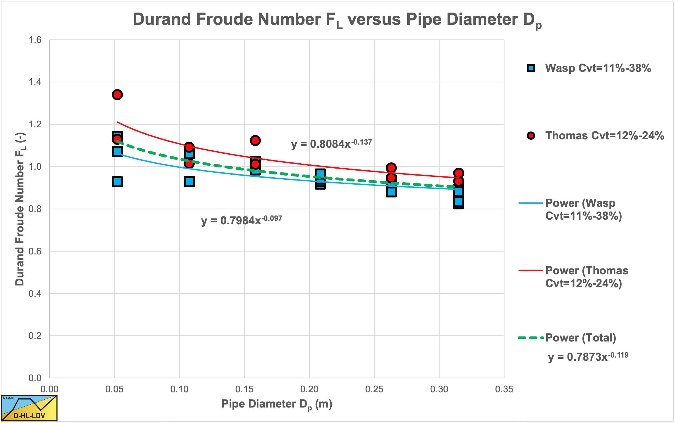
Both Wasp et al. (1977) and A.D. Thomas (1979) reported LDV values in pipes with diameters ranging from 0.05 m to 0.3 m (2-12 inch) for a d=0.18 mm sand. The resulting Durand Froude numbers are shown in Figure 6.19-1. In both cases the FL value decreases slightly with increasing pipe diameter to a power of about -0.1. The scatter in the graph is mainly due to different volumetric concentrations.

Table 6.19-1: 6 implementations of the WASP model.

Model	Friction Velocity	Argument Suspended Fraction	Vehicle Hydraulic Gradient	Solids Hydraulic Gradient
Wasp	\(\ \mathrm{u}_{*}=\sqrt{\frac{\mathrm{i}_{\mathrm{t o t a l}} \cdot \mathrm{g} \cdot \mathrm{D}_{\mathrm{p}}}{\mathrm{4}} \cdot \frac{\rho_{\mathrm{l}}}{\rho_{\mathrm{v}}}}\)	\(\ \frac{\mathrm{v}_{\mathrm{t} \mathrm{v}}}{\mathrm{1} \cdot \kappa \cdot \mathrm{u}_{*}}\)	\(\ \mathrm{i}_{\mathrm{v} \mathrm{e h i c l e}}=\frac{\rho_{\mathrm{v}}}{\rho_{\mathrm{l}}} \cdot \mathrm{i}_{\mathrm{l} \mathrm{v}}\)	\(\ \mathrm{i}_{\mathrm{D u}}=\mathrm{i}_{\mathrm{l}} \cdot \mathrm{D} \mathrm{u}\)
Lahiri & Ni	\(\ \mathrm{u}_{*}=\sqrt{\frac{\mathrm{i}_{\mathrm{v e h i c l e}} \cdot \mathrm{g} \cdot \mathrm{D}_{\mathrm{p}}}{4}}\)	\(\ \frac{\mathrm{v}_{\mathrm{t}} \cdot\left(\mathrm{1}-\mathrm{C}_{\mathrm{v s}}\right)^{\beta}}{\mathrm{1} \cdot \mathrm{\kappa} \cdot \mathrm{u}_{*}}\)	\(\ \mathrm{i}_{\mathrm{v e h i c l e}}=\frac{\rho_{\mathrm{v}}}{\rho_{\mathrm{l}}} \cdot \mathrm{i}_{\mathrm{l}}\)	\(\ \mathrm{i}_{\mathrm{D u}}=\frac{\rho_{\mathrm{v}}}{\rho_{\mathrm{l}}} \cdot \mathrm{i}_{\mathrm{l}} \cdot \mathrm{D} \mathrm{u}\)
Kaushal A	\(\ \mathrm{u}_{*}=\sqrt{\frac{\mathrm{i}_{\mathrm{t} \mathrm{o} \mathrm{t a l}} \cdot \mathrm{g} \cdot \mathrm{D}_{\mathrm{p}}}{\mathrm{4}}}\)	\(\ \frac{\mathrm{v}_{\mathrm{t}} \cdot\left(\mathrm{1}-\mathrm{C}_{\mathrm{v s}}\right)^{\beta}}{\beta_{\mathrm{sm}, \text { Kaushal }} \cdot \kappa \cdot \mathrm{u}_{*}}\)	\(\ \mathrm{i}_{\text {vehicle }}=\frac{\rho_{\mathrm{v}}}{\rho_{\mathrm{l}}} \cdot \mathrm{i}_{\mathrm{l}}\)	\(\ \mathrm{i}_{\mathrm{D u}}=\mathrm{i}_{\mathrm{l}} \cdot \mathrm{D} \mathrm{u}\)
Kaushal B	\(\ \mathrm{u}_{*}=\sqrt{\frac{\mathrm{i}_{\mathrm{t} \mathrm{o} \mathrm{t a l}} \cdot \mathrm{g} \cdot \mathrm{D}_{\mathrm{p}}}{\mathrm{4}}}\)	\(\ \frac{\mathrm{v}_{\mathrm{t}} \cdot\left(\mathrm{1}-\mathrm{C}_{\mathrm{v} \mathrm{s}}\right)^{\beta}}{\mathrm{1} \cdot \mathrm{\kappa} \cdot \mathrm{u}_{*}}\)	\(\ \mathrm{i}_{\text {vehicle }}=\frac{\rho_{\mathrm{v}}}{\rho_{\mathrm{l}}} \cdot \mathrm{i}_{\mathrm{l}}\)	\(\ \mathrm{i}_{\mathrm{D u}}=\mathrm{i}_{\mathrm{l}} \cdot \mathrm{D} \mathrm{u}\)
Abulnaga	\(\ \mathrm{u}_{*}=\sqrt{\frac{\mathrm{i}_{\mathrm{t} \mathrm{o} \mathrm{t a l}} \cdot \mathrm{g} \cdot \mathrm{D}_{\mathrm{p}}}{\mathrm{4}}}\)	\(\ \frac{\mathrm{v}_{\mathrm{t}} \cdot\left(\mathrm{1}-\mathrm{C}_{\mathrm{v} \mathrm{s}}\right)^{\beta}}{\mathrm{1} \cdot \mathrm{\kappa} \cdot \mathrm{u}_{*}}\)	\(\ \mathrm{i}_{\text {vehicle }}=\frac{\rho_{\mathrm{m}}}{\rho_{\mathrm{l}}} \cdot \mathrm{i}_{\mathrm{l}}\)	\(\ \mathrm{i}_{\mathrm{D u}}=\frac{\rho_{\mathrm{m}}}{\rho_{\mathrm{l}}} \cdot \mathrm{i}_{\mathrm{l}} \cdot \mathrm{D} \mathrm{u}\)
DHLLDV	\(\ \mathrm{u}_{*}=\sqrt{\frac{\mathrm{i}_{\mathrm{v} \mathrm{e h i c l e}} \cdot \mathrm{g} \cdot \mathrm{D}_{\mathrm{p}}}{4} \cdot \frac{\rho_{\mathrm{l}}}{\rho_{\mathrm{v}}}}\)	\(\ \frac{\alpha_{\mathrm{sm}}}{\mathrm{C}_{\mathrm{vr}}} \cdot \frac{\mathrm{u}_{*},_{ \mathrm{ldv}}}{\mathrm{u}_{*}} \cdot \frac{\mathrm{v}_{\mathrm{tv}}}{\mathrm{v}_{\mathrm{tv}, \mathrm{ldv}}}\)	\(\ \mathrm{i}_{\mathrm{v e h i c l e}}=\frac{\rho_{\mathrm{v}}}{\rho_{\mathrm{l}}} \cdot \mathrm{i}_{\mathrm{l v}}\)	\(\ \mathrm{i}_{\mathrm{D u}}=\mathrm{i}_{\mathrm{l}} \cdot \mathrm{D u}\)

Figure 6.19-1: Durand Froude number F_L versus pipe diameter D_p for a d=0.18 mm sand.

Here the transport concentration is used, because the experimental data was based on the transport concentration.

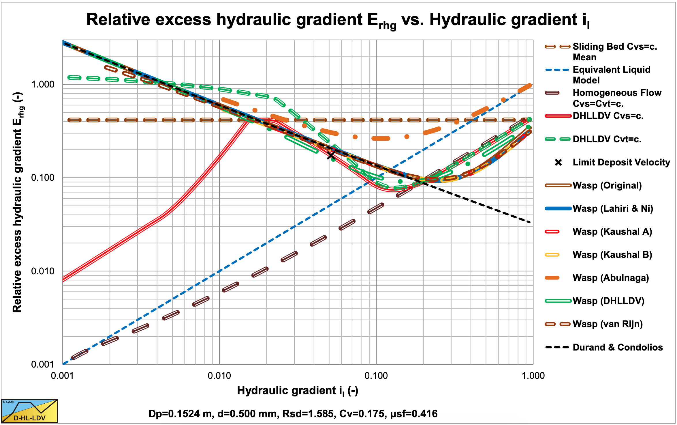
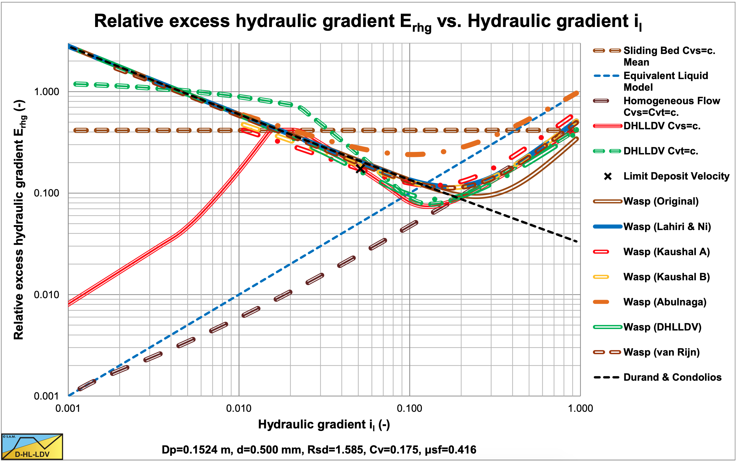
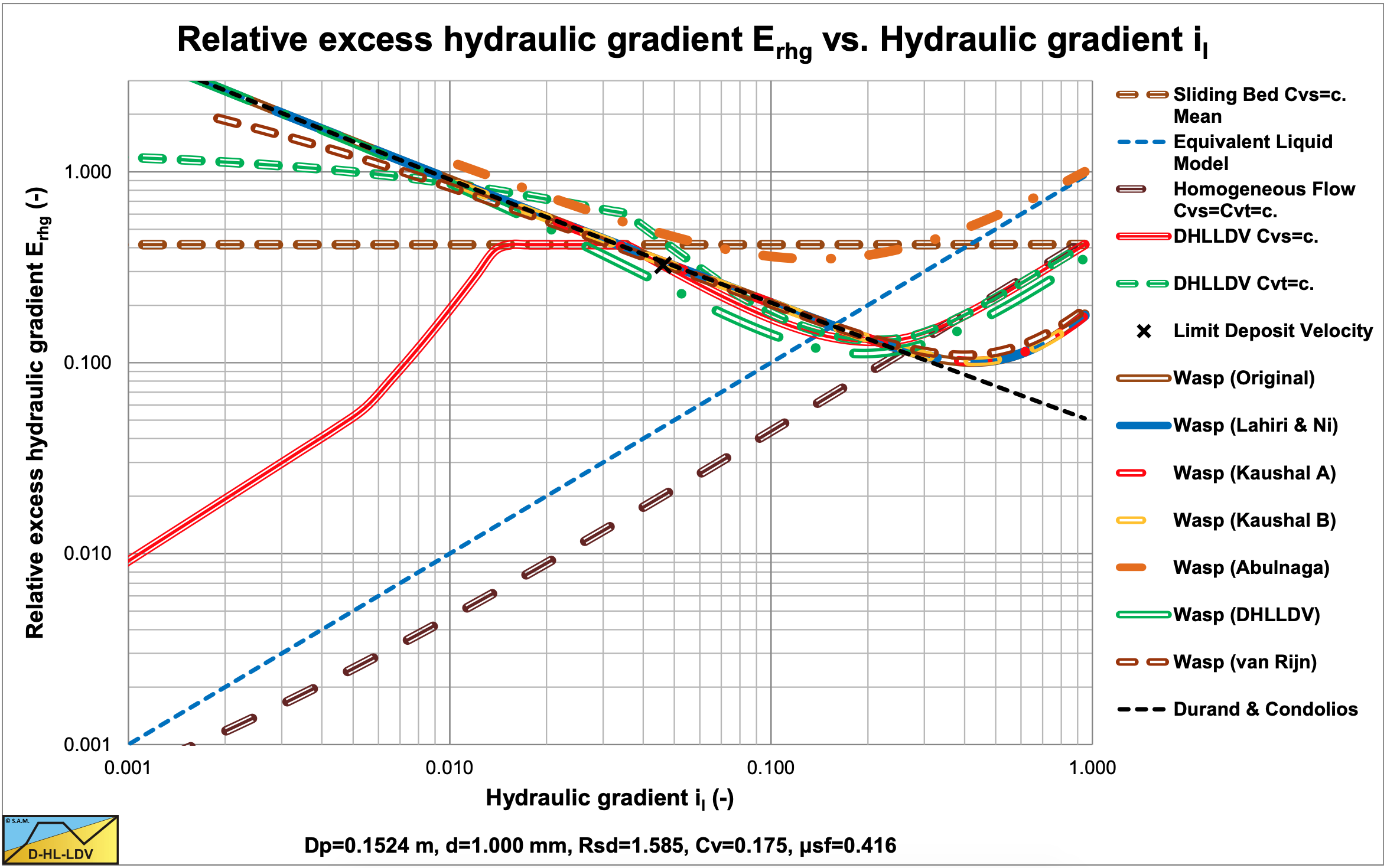
Figure 6.19-2, Figure 6.19-6, Figure 6.19-10 and Figure 6.19-14 show the results of 6 different approaches of the Wasp model for 4 uniform sands. Here the diffusivities are used as in the original Wasp model and hindered settling is not applied. The Kaushal & Tomita (2002B) and the Lahiri (2009) approach give an almost equal result. Apparently it does not make a lot of difference whether the bed portion is multiplied with the pure liquid or the vehicle hydraulic gradient. The Abulnaga (2002) approach gives a very different result, due to the multiplication with the mixture density. For small particle diameters the results are close to the ELM and the DHLLDV Frameworks.

Figure 6.19-2: The Wasp model for a d=0.1 mm sand particle.

Figure 6.19-3: The Wasp model for a d=0.1 mm sand particle, modified diffusivity and hindered settling.

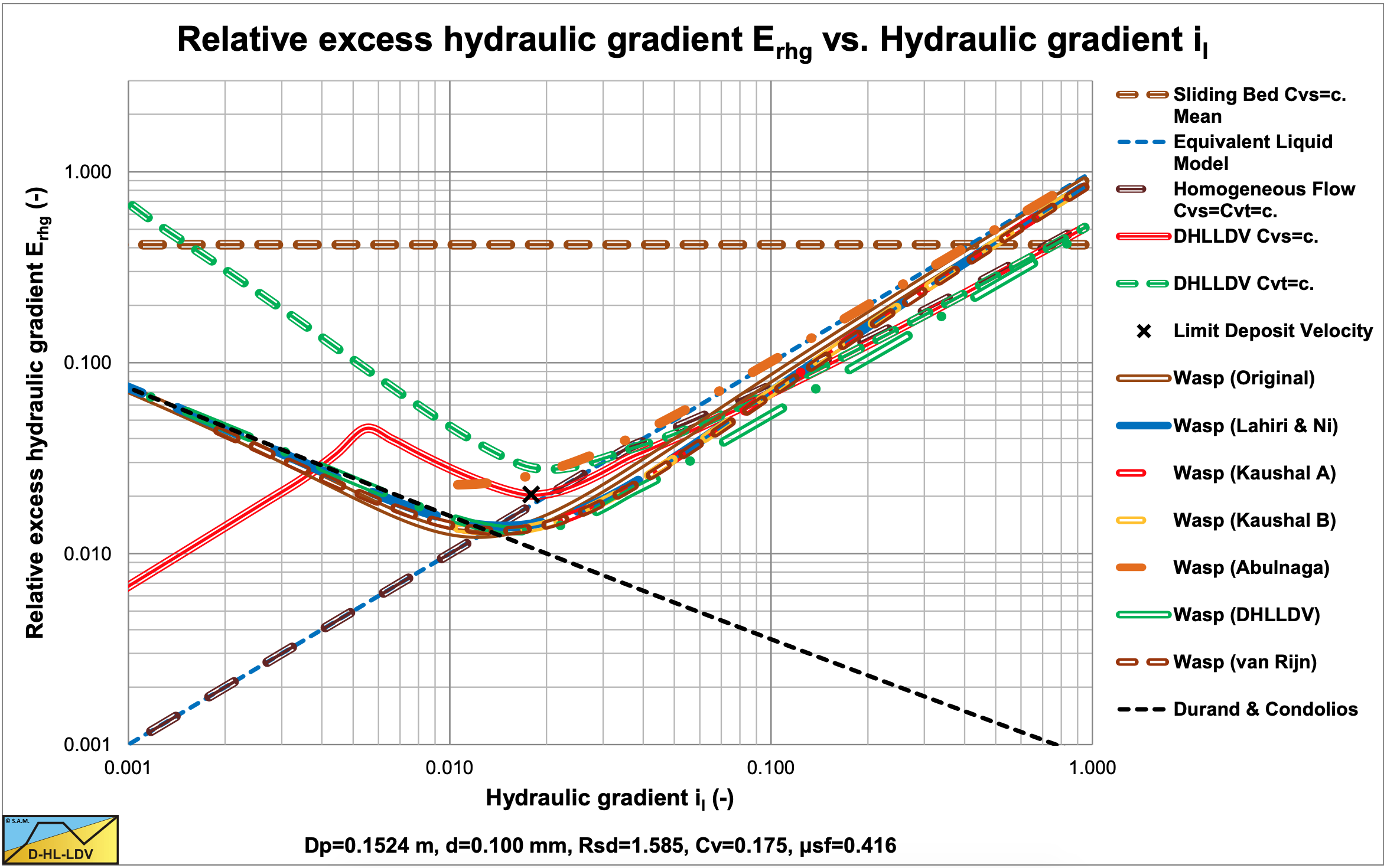
For the larger particles however the Kaushal & Tomita (2002B) and the Lahiri (2009) approaches (the assumed original Wasp model) underestimate pressure losses compared to the ELM at higher line speeds.

Figure 6.19-4: The suspended fraction for a d=0.1 mm sand particle.

Figure 6.19-5: The suspended fraction for a d=0.1 mm sand particle, modified diffusivity and hindered settling.

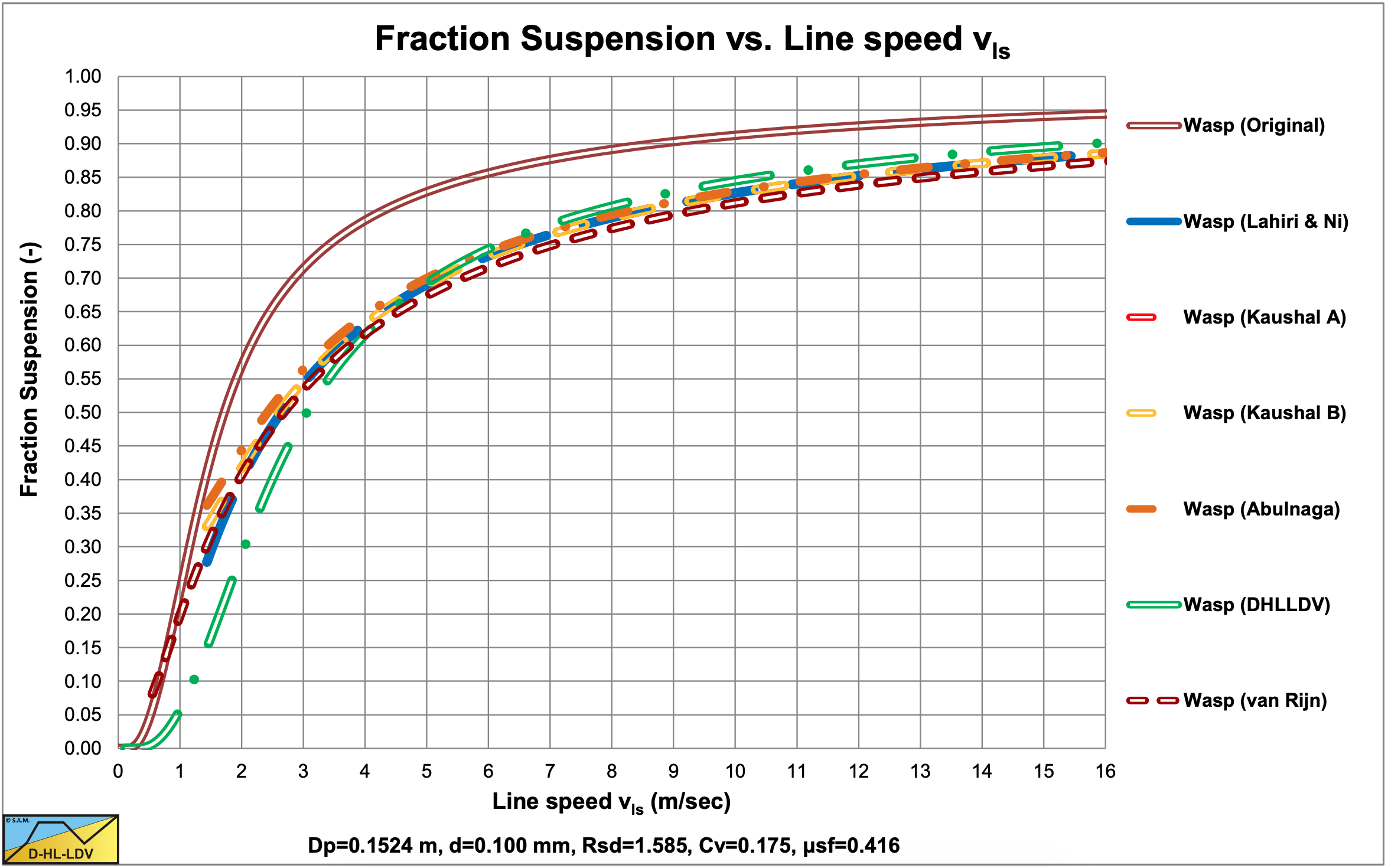
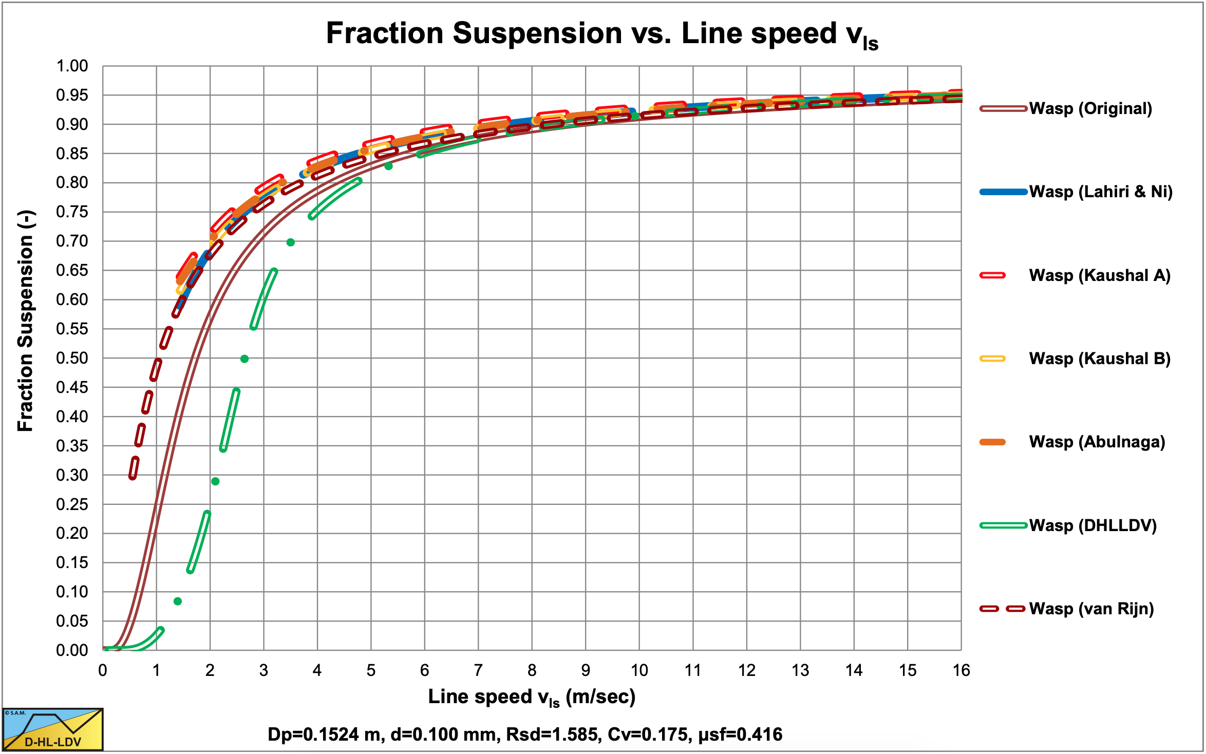
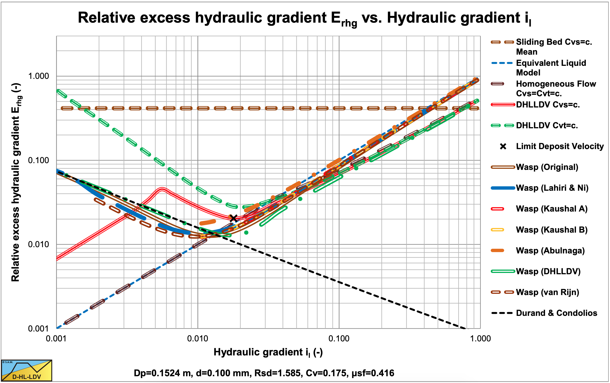
Figure 6.19-3, Figure 6.19-7, Figure 6.19-11 and Figure 6.19-15 show the results with hindered settling applied for all 6 approaches. The Kaushal & Tomita (2002B) method also includes their modified diffusivity (Kaushal A). In all cases the curves are closer to the ELM curve, especially for the small particles. Hindered settling and an increased diffusivity increase the solids fraction in the vehicle and decrease the solids fraction in the bed. The Durand factor, equation (6.19-22) is not affected however. A hydraulic gradient of 0.1 on the abscissa is equivalent to a line speed of 5 m/sec, a line speed of normal operation for the pipe diameter of 0.1524 m.

Figure 6.19-6: The Wasp model for a d=0.2 mm sand particle.

Figure 6.19-7: The Wasp model for a d=0.2 mm sand particle, modified diffusivity and hindered settling.

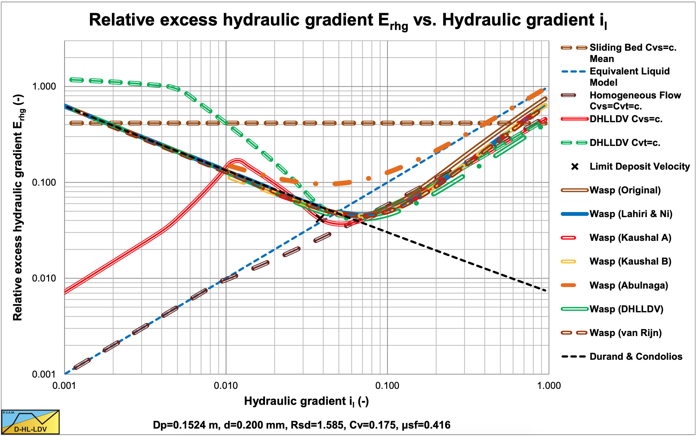
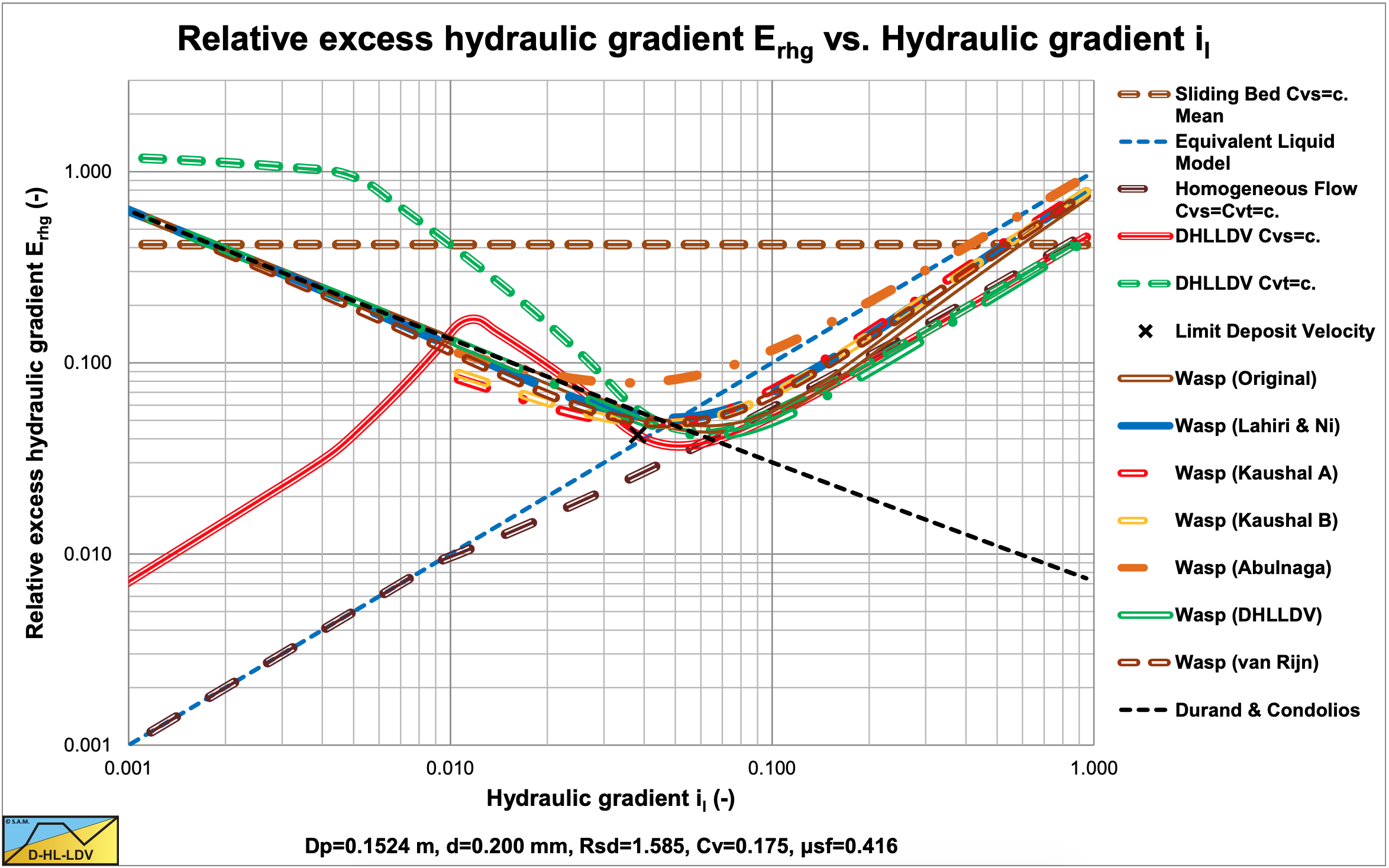
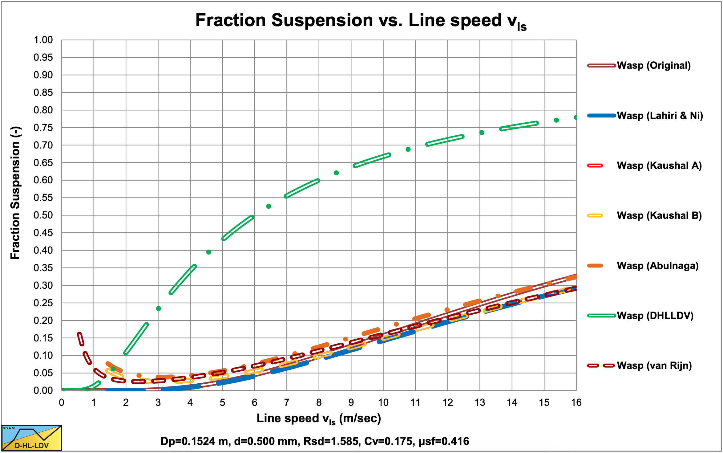
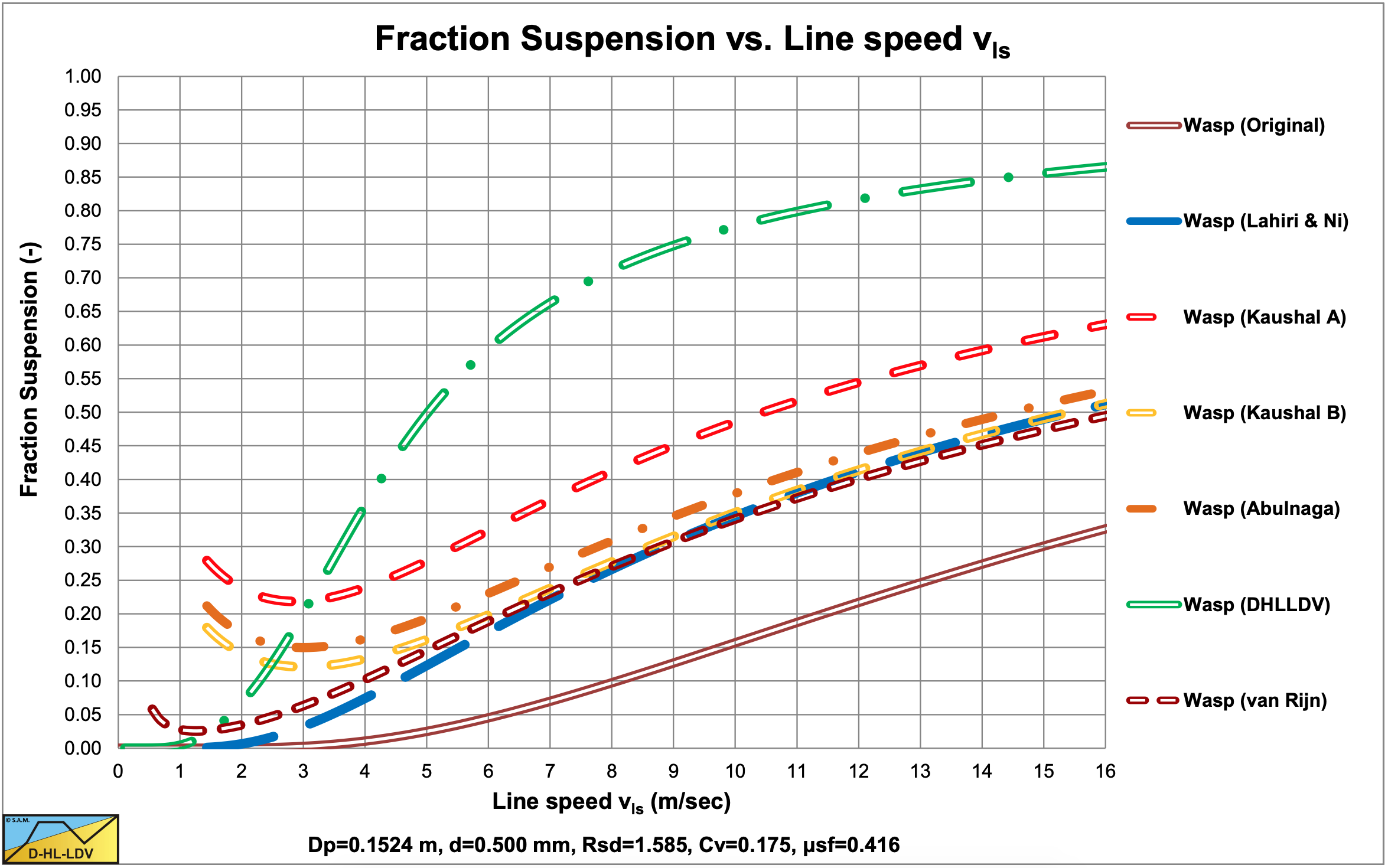
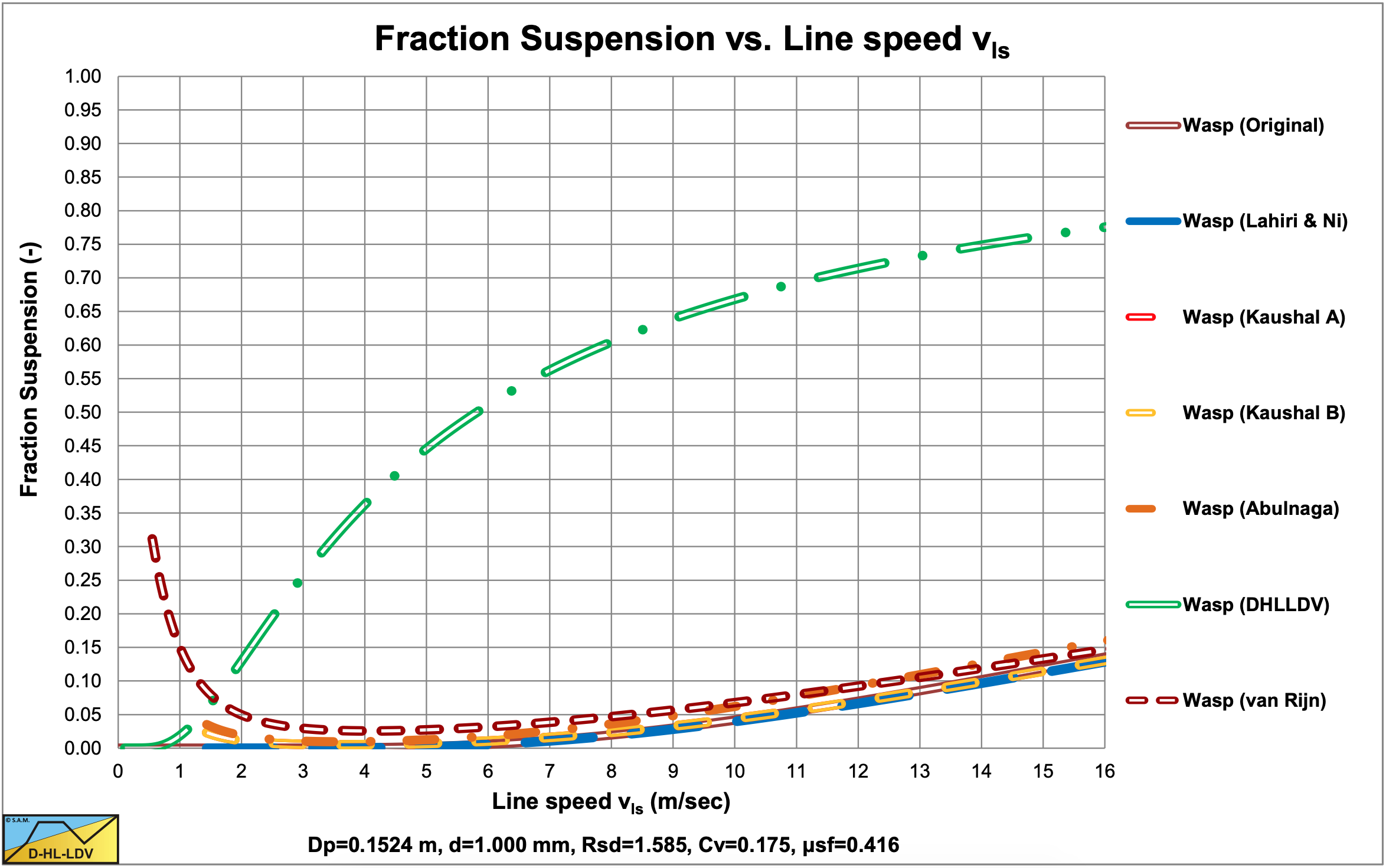
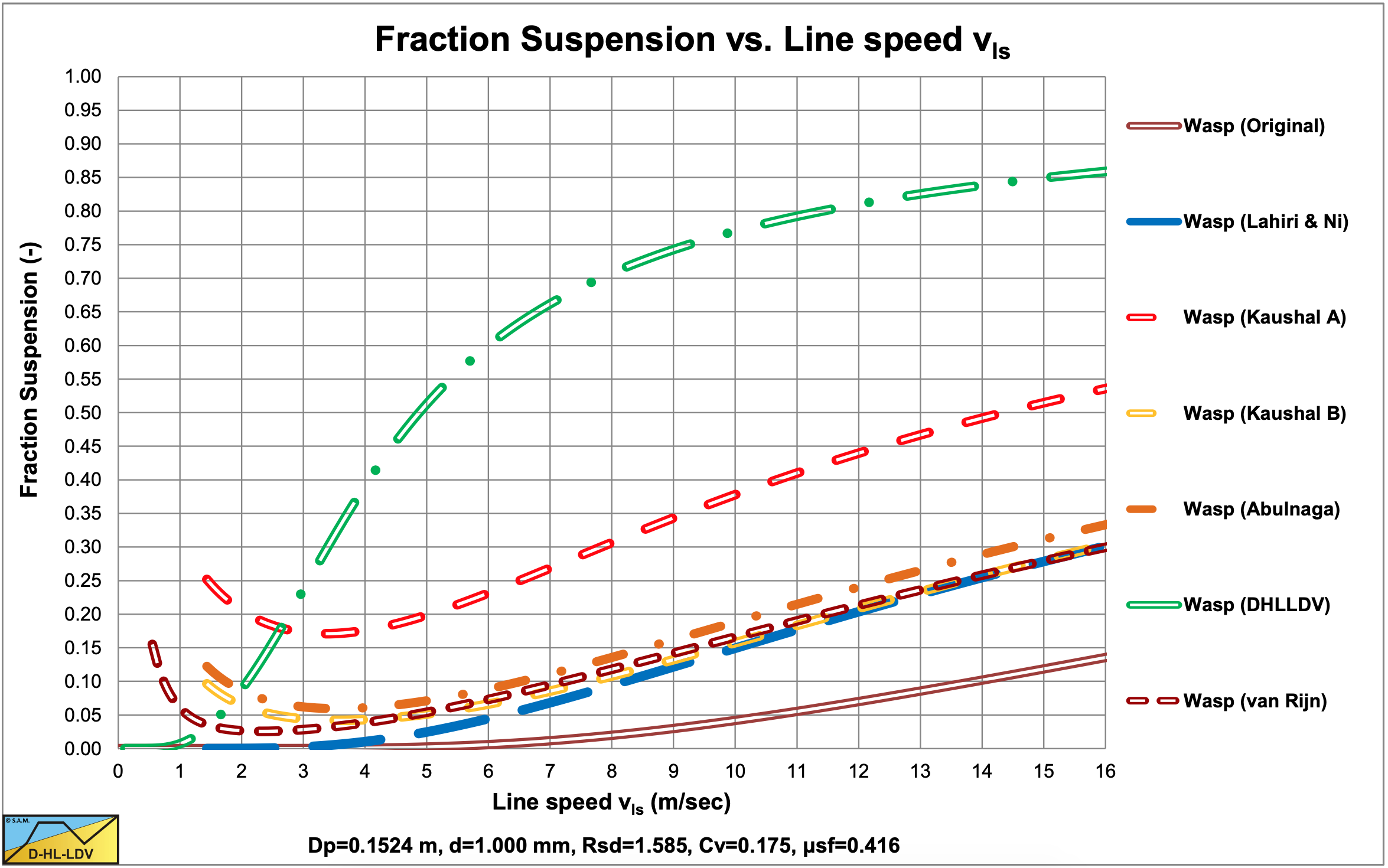
Figure 6.19-4, Figure 6.19-8, Figure 6.19-12 and Figure 6.19-16 show the suspended fraction for all 6 implementations, without hindered settling and modified diffusivity. Figure 6.19-5, Figure 6.19-9, Figure 6.19-13 and Figure 6.19-17 show the suspended fraction for all 6 implementations, with hindered settling (all) and modified diffusivity (Kaushal A). It is clear that both hindered settling and the modified diffusivity increase the suspended fraction. The DHLLDV implementation and the Kaushal A implementation with modified diffusivity give about the same suspended fraction for higher line speeds. The DHLLDV implementation gives a higher suspended fraction for larger particles. This is the result of using a diffusivity based on the LDV.

Figure 6.19-10: The Wasp model for a d=0.5 mm sand particle.

Figure 6.19-11: The Wasp model for a d=0.5 mm sand particle, modified diffusivity and hindered settling.

Figure 6.19-12: The suspended fraction for a d=0.5 mm sand particle.

Figure 6.19-13: The suspended fraction for a d=0.5 mm sand particle, modified diffusivity and hindered settling.

The DHLLDV implementation does depend on hindered settling due to its definition of the diffusivity. The model is consistent in itself relating the diffusivity to the LDV in such a way that at the LDV the bottom concentration equals the bed concentration. At higher line speeds the bottom concentration will be lower than the bed concentration. Hindered settling does affect the LDV and the settling velocity, so implicitly the DHLLDV solution depends on hindered settling. Here the DHLLDV implementation is a combination of the Durand & Condolios (1952) model and the ELM. In chapter 7 the combination of DHLLDV and ELM is discussed.

Effectively, both hindered settling and an increased diffusivity, have the effect of reducing the value of the argument in equation (6.19-15), acting like the settling velocity and thus the particle diameter are much smaller. Small particles tend to behave according to the ELM at line speeds high enough. At low line speeds however this effect is limited and the curves behave according to the Durand & Condolios (1952) equation.

Figure 6.19-14: The Wasp model for a d=1.0 mm sand particle.

Figure 6.19-15: The Wasp model for a d=1.0 mm sand particle, modified diffusivity and hindered settling.

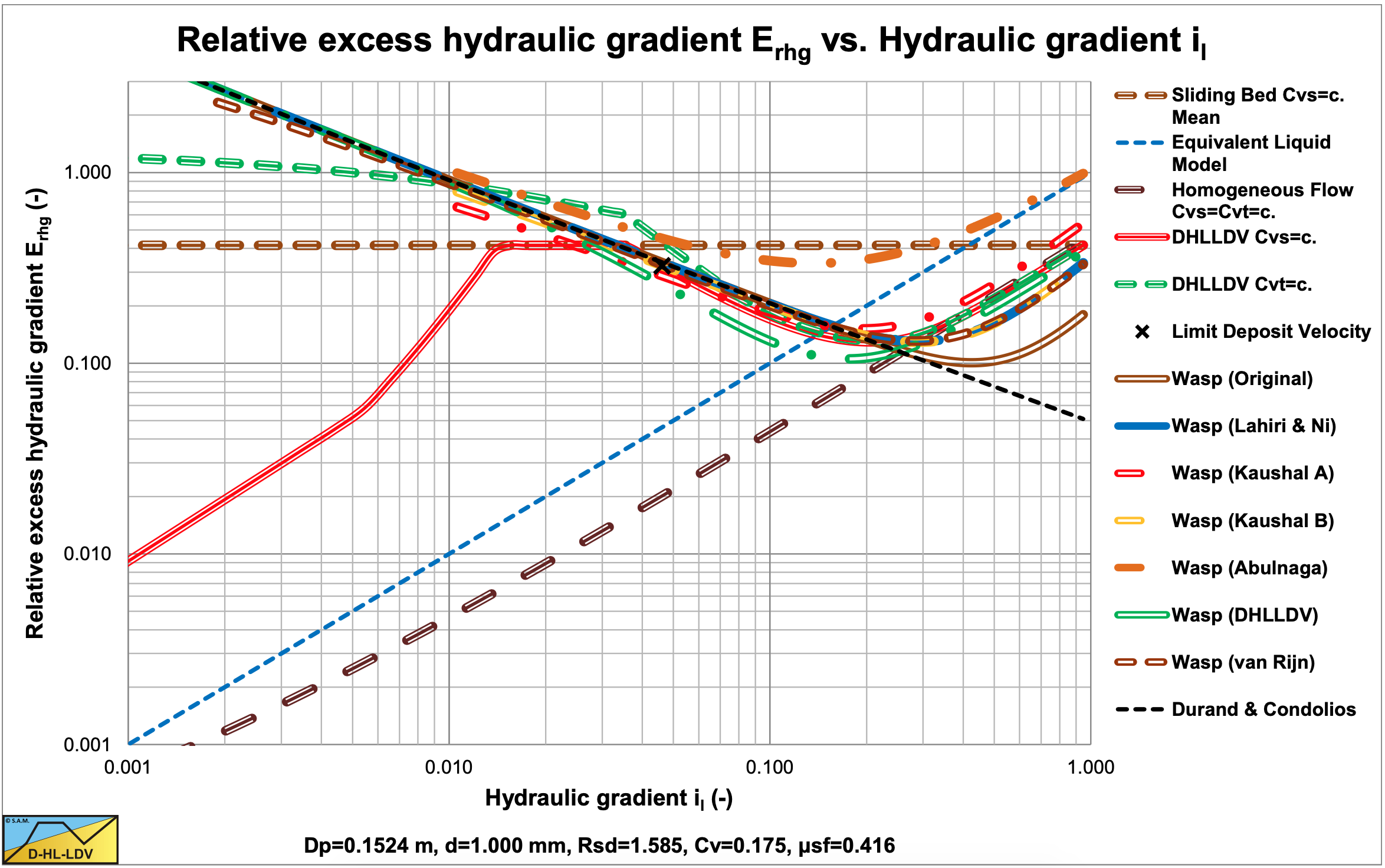
A combination of the Durand & Condolios (1952) equation (or any equation for the heterogeneous regime) for low line speeds and the ELM model with a reduction factor for line speeds above the intersection point, would give the same result. However especially the Kaushal & Tomita (2002B) method gives valuable additional information regarding the concentration profile in the pipe. The DHLLDV approach gives almost the same resulting hydraulic gradient as the Kaushal & Tomita (2002B) approach, both with hindered settling and the latter with modified diffusivity. For particles larger than d>0.015·D_p, the WASP method underestimates the hydraulic gradient in all cases, except the Abulnaga (2002) approach.

Figure 6.19-16: The suspended fraction for a d=1.0 mm sand particle.

Figure 6.19-17: The suspended fraction for a d=1.0 mm sand particle, modified diffusivity and hindered settling.

6.19.5 Nomenclature Wasp Model

Cvt	Delivered/transport volumetric concentration	-
Cvs	Spatial volumetric concentration	-
Cvs,j	Spatial volumetric concentration, j^th fraction	-
Cvs,v	Spatial volumetric concentration vehicle (homogeneous fraction)	-
Cvs,v,j	Spatial volumetric concentration vehicle (homogeneous fraction), j^th fraction	-
Cvs,Du	Spatial volumetric concentration Durand fraction (heterogeneous fraction)	-
Cvc,Du,j	Spatial volumetric concentration Durand fraction (heterogeneous fraction), j^th fraction	-
Ctop	Spatial volumetric concentration at 92% of the pipe diameter, from the bottom of the pipe	-
Ccenter	Spatial volumetric concentration at 50% of the pipe diameter, from the bottom of the pipe	-
Cvb	Spatial volumetric concentration bed	-
CvB	Spatial volumetric concentration bottom of pipe	-
CD	Particle drag coefficient	-
CD,j	Particle drag coefficient j^th fraction	-
Cx	Durand & Condolios reversed particle Froude number squared	-
Cx,j	Durand & Condolios reversed particle Froude number squared j^th fraction	-
d	Particle diameter	-
dj	Particle diameter j^th fraction	m
dm	Mean particle diameter, Kaushal & Tomita	m
dmw	Weighed mean particle diameter, Kaushal & Tomita	m
Dp	Pipe diameter	m
Du	Durand & Condolios factor	-
Duj	Durand & Condolios factor j^th fraction	-
Erhg	Relative excess hydraulic gradient	-
fm	Fanning friction factor mixture, Kaushal & Tomita	-
FL	Durand & Condolios LDV Froude number	-
Frp	Particle Froude number	-
Frp,j	Particle Froude number j^th fraction	-
g	Gravitational constant 9.81 m/s^2	m/s^2
i	Hydraulic gradient	-
il	Hydraulic gradient pure liquid	-
ibed	Hydraulic gradient bed, Kaushal & Tomita	-
ibed,j	Hydraulic gradient bed j^th fraction, Kaushal Tomita	-
ivehicle, ilv	Hydraulic gradient vehicle	-
iDu	Hydraulic gradient heterogeneous transport	-
iDu,j	Hydraulic gradient heterogeneous transport, contribution j^thfraction	-
itotal	Total hydraulic gradient, homogeneous plus heterogeneous	-
j	Fraction number	-
ΔL	Length of pipeline	m
LDV	Limit Deposit Velocity	m/s
n	Number of fractions	-
Δptotal	Total pressure drop	kPa
r	Position in the pipe, from the bottom of the pipe	m
Re	Reynolds number	-
Rel	Reynolds number based on pure liquid properties	-
Rev	Reynolds number based on vehicle properties	-
Rsd	Relative submerged density solids in pure liquid	-
Rsd,v	Relative submerged density solids in vehicle	-
u*	Friction velocity	m/s
u*,ldv	Friction velocity at LDV	m/s
vls	Line speed	m/s
vls,ldv	Limit Deposit Velocity	m/s
vt	Terminal settling velocity in pure liquid	m/s
vtv	Terminal settling velocity in the vehicle	m/s
vtv,j	Terminal settling velocity in the vehicle of the j^th fraction	m/s
vtv,ldv	Terminal settling velocity in the vehicle at LDV	m/s
αsm	Correction factor Relation sediment diffusivity – eddy momentum diffusivity	-
βsm	Relation sediment diffusivity – eddy momentum diffusivity	-
βsm,Kaushal	Relation sediment diffusivity – eddy momentum diffusivity, Kaushal & Tomita	-
βsm,ldv	Relation sediment diffusivity – eddy momentum diffusivity, DHLLDV	-
ε	Pipe wall roughness	m
εs	Sediment diffusivity	m/s
κ	Von Karman constant, about 0.4	-
λl	Darcy Weisbach friction factor based on liquid properties	-
λm	Darcy Weisbach friction factor mixture, Kaushal & Tomita	-
λv	Darcy Weisbach friction factor based on vehicle properties	-
λv,new	Corrected Darcy Weisbach friction factor Abulnaga	-
λe	Effective Darcy Weisbach friction factor based on total hydraulic gradient	-
ρl	Density liquid	ton/m^3
ρs	Density solids	ton/m^3
ρm	Density mixture	ton/m^3
ρv	Density vehicle	ton/m^3
σg	PSD grading coefficient, Kaushal & Tomita	-
μl	Dynamic viscosity liquid	Pa·s
μv	Dynamic viscosity vehicle	Pa·s
μr	Relative dynamic viscosity vehicle	-
μsf	Sliding friction factor	-
\(\ v_{\mathbf{l}}\)	Kinematic viscosity pure liquid	m^2/s
\(\ v_{\mathbf{v}}\)	Kinematic viscosity vehicle	m^2/s