6.17: The Wilson-GIW (1979) Models

6.20.1 The Wilson-GIW (1979) Model for Fully Stratified Flow

6.20.1.1 Introduction

The Wilson et al. (1992), (1997) and (2006) model for the hydraulic transport of solids in pipelines is a widely used model for the sliding bed regime. A theoretical background of the model has been published piece by piece in a number of articles over the years. A variety of information provided in these publications makes the model difficult to reconstruct. Wilson (1979) first published his theory in 1979. Riet et al. (1995) & (1996) and Miedema et al. (2002) tried to reproduce the Wilson (1979) model.

A good understanding of the model structure is inevitable for the user who wants to extend or adapt the model to specific slurry flow conditions. The aim of this chapter is to summarize the model theory and submit the results of the numerical analysis carried out on the various model configurations. The numerical results show some differences when compared with the nomographs presented in the literature as the graphical presentations of the generalised model outputs. Model outputs are sensitive on a number of input parameters and on a model configuration used. This chapter contains an overview of a theory of the Wilson et al. (1992) two-layer model (2LM) as it has been published in a number of articles over the years. Results are presented from the model computation. The results provide an insight to the behavior of the mathematical model.

The model is based on an equilibrium of forces acting on the bed. Driving forces and resisting forces can be distinguished. The driving forces on the bed are the shear forces on the top of the bed and the force resulting from the pressure times the bed cross section. The pressure is the result of the sum of the shear force on the pipe wall in the restricted area above the bed and the shear force on the bed, divided by the cross section of this restricted area. The resisting forces are the force as a result of the sliding friction between the bed and the pipe wall and the viscous friction force of the liquid between the particles in the bed and the pipe wall. When the sum of the driving forces equals the sum of the resisting forces, the so called Limit of Stationary Deposit Velocity is reached. At line speeds below the Limit of Stationary Deposit Velocity, the bed is stationary and does not move, because the driving forces are smaller than the maximum resisting forces (maximum if the sliding friction would be fully mobilized, which is not the case at line speeds below the Limit of Stationary Deposit Velocity). At line speeds above the Limit of Stationary Deposit Velocity, the bed is sliding with a speed that is increasing with increasing line speed.

6.20.1.2 The Basic Equations for Flow and Geometry

In order to understand the model, first all the geometrical parameters are defined. The cross section of the pipe with a particle bed as defined in the Wilson et al. (1992) two layer model has been illustrated by Figure 6.20-1.

Figure 6.20-1: The definitions for fully stratified flow.

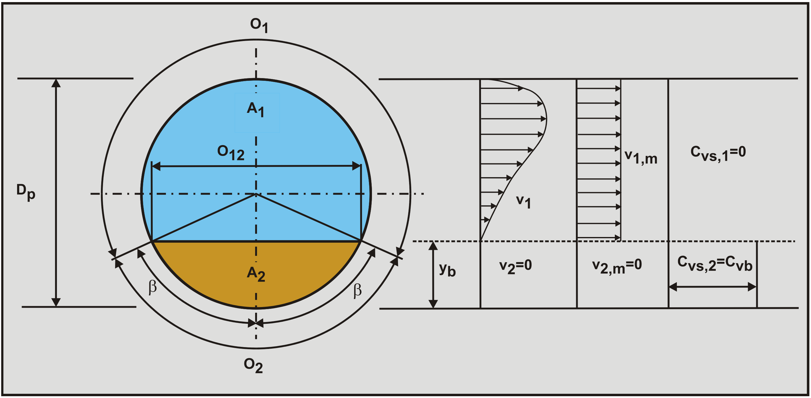
The geometry is defined by the following equations.

The length of the liquid in contact with the whole pipe wall if there is no bed is:

\[\ \mathrm{O}_{\mathrm{p}}=\pi \cdot \mathrm{D}_{\mathrm{p}}\]

The length of the liquid or the suspension in contact with the pipe wall:

\[\ \mathrm{O}_{1}=\mathrm{D}_{\mathrm{p}} \cdot(\pi-\beta)\]

The length of the fixed or sliding bed in contact with the wall:

\[\ \mathrm{O}_{2}=\mathrm{D}_{\mathrm{p}} \cdot \boldsymbol{\beta}\]

The top surface length of the fixed or sliding bed:

\[\ \mathrm{O}_{12}=\mathrm{D}_{\mathrm{p}} \cdot \sin (\beta)\]

The cross sectional area A_p of the pipe is:

\[\ \mathrm{A}_{\mathrm{p}}=\frac{\pi}{4} \cdot \mathrm{D}_{\mathrm{p}}^{\mathrm{2}}\]

The cross sectional area A₂ of the fixed or sliding bed is:

\[\ \mathrm{A}_{2}=\frac{\pi}{4} \cdot \mathrm{D}_{\mathrm{p}}^{2} \cdot\left(\frac{\boldsymbol{\beta}-\sin (\beta) \cdot \cos (\beta)}{\pi}\right)\]

The cross sectional area A₁ above the bed, where the liquid or the suspension is flowing, also named the restricted area:

\[\ \mathrm{A}_{\mathrm{1}}=\mathrm{A}_{\mathrm{p}}-\mathrm{A}_{2}\]

The hydraulic diameter of the cross-section of the pipeline above the bed D_H as function of the bed height, is equal to four times the cross sectional area divided by the wetted perimeter:

\[\ \mathrm{D}_{\mathrm{H}, \mathrm{1}}=\frac{\mathrm{4} \cdot \mathrm{A}_{\mathrm{1}}}{\mathrm{O}_{\mathrm{1}}+\mathrm{O}_{\mathrm{1 2}}} \quad\text{ or simplified: }\quad \mathrm{D}_{\mathrm{H}, \mathrm{1}}=\sqrt{\frac{\mathrm{4} \cdot \mathrm{A}_{\mathrm{1}}}{\pi}}\]

The volume balance gives a relation between the line speed v_ls, the velocity in the restricted area above the bed v_r or v₁ and the velocity of the bed v_b or v₂.

\[\ \mathrm{v}_{\mathrm{l s}} \cdot \mathrm{A}_{\mathrm{p}}=\mathrm{v}_{\mathrm{1}} \cdot \mathrm{A}_{\mathrm{1}}+\mathrm{v}_{2} \cdot \mathrm{A}_{2}\]

Thus the velocity in the restricted area above the bed is:

\[\ \mathrm{v}_{1}=\frac{\mathrm{v}_{\mathrm{l s}} \cdot \mathrm{A}_{\mathrm{p}}-\mathrm{v}_{2} \cdot \mathrm{A}_{2}}{\mathrm{A}_{1}}\]

Or the velocity of the bed is:

\[\ \mathrm{v}_{2}=\frac{\mathrm{v}_{\mathrm{l} \mathrm{s}} \cdot \mathrm{A}_{\mathrm{p}}-\mathrm{v}_{\mathrm{1}} \cdot \mathrm{A}_{\mathrm{1}}}{\mathrm{A}_{2}}\]

6.20.1.3 The Shear Stresses Involved

In order to determine the forces involved, first the shear stresses involved have to be determined. The general equation for the shear stresses is:

\[\ \tau=\rho_{1} \cdot \mathrm{u}_{*}^{2}=\frac{\lambda_{\mathrm{l}}}{4} \cdot \frac{1}{2} \cdot \rho_{1} \cdot \mathrm{v}^{2}\]

The force F on the pipe wall over a length ΔL is now:

\[\ \mathrm{F}=\tau \cdot \pi \cdot \mathrm{D}_{\mathrm{p}} \cdot \Delta \mathrm{L}=\frac{\lambda_{\mathrm{l}}}{\mathrm{4}} \cdot \frac{\mathrm{1}}{2} \cdot \rho_{\mathrm{l}} \cdot \mathrm{v}^{2} \cdot \pi \cdot \mathrm{D}_{\mathrm{p}} \cdot \Delta \mathrm{L}\]

The pressure Δp required to push the solid-liquid mixture through the pipe equals the force divided by the cross-section:

\[\ \Delta \mathrm{p}=\frac{\mathrm{F}}{\mathrm{A}_{\mathrm{p}}}=\frac{\frac{\lambda_{\mathrm{l}}}{\mathrm{4}} \cdot \frac{\mathrm{1}}{2} \cdot \rho_{\mathrm{l}} \cdot \mathrm{v}^{2} \cdot \pi \cdot \mathrm{D}_{\mathrm{p}} \cdot \Delta \mathrm{L}}{\frac{\pi}{4} \cdot \mathrm{D}_{\mathrm{p}}^{2}}=\lambda_{\mathrm{l}} \cdot \frac{\Delta \mathrm{L}}{\mathrm{D}_{\mathrm{p}}} \cdot \frac{\mathrm{1}}{2} \cdot \rho_{\mathrm{l}} \cdot \mathrm{v}^{2}\]

This is the well-known Darcy Weisbach equation. Over the whole range of Reynolds numbers above 2320 (5000<Re<100.000) the Swamee Jain equation gives a good approximation for the friction coefficient:

\[\ \lambda_{\mathrm{l}}=\frac{1.325}{\left(\ln \left(\frac{0.27 \cdot \varepsilon}{\mathrm{D}_{\mathrm{p}}}+\frac{5.75}{\mathrm{Re}^{0.9}}\right)\right)^{2}} \quad \text{ with: }\quad \mathrm{Re}=\frac{\mathrm{v} \cdot \mathrm{D}_{\mathrm{p}}}{v_{\mathrm{l}}}\]

This gives for the shear stress on the pipe wall for clean water:

\[\ \tau_{\mathrm{l}}=\frac{\lambda_{\mathrm{l}}}{4} \cdot \frac{1}{2} \cdot \rho_{\mathrm{l}} \cdot \mathrm{v}_{ \mathrm{ls}}^{2} \quad\text{ with: }\quad \lambda_{\mathrm{l}}=\frac{1.325}{\left(\ln \left(\frac{0.27 \cdot \varepsilon}{\mathrm{D}_{\mathrm{p}}}+\frac{5.75}{\mathrm{Re}^{0.9}}\right)\right)^{2}} \quad\text{ and }\quad \mathrm{Re}=\frac{\mathrm{v}_{\mathrm{ls}} \cdot \mathrm{D}_{\mathrm{p}}}{v_{\mathrm{l}}}\]

For the flow in the restricted area, the shear stress between the liquid and the pipe wall is:

\[\ \tau_{1,\mathrm{l}}=\frac{\lambda_{1}}{4} \cdot \frac{1}{2} \cdot \rho_{\mathrm{l}} \cdot \mathrm{v}_{1}^{2} \quad\text{ with: }\quad \lambda_{1}=\frac{1.325}{\left(\ln \left(\frac{0.27 \cdot \varepsilon}{\mathrm{D}_{\mathrm{H}, 1}}+\frac{5.75}{\mathrm{R} \mathrm{e}^{0.9}}\right)\right)^{2}} \quad\text{ and }\quad \mathrm{R} \mathrm{e}=\frac{\mathrm{v}_{1} \cdot \mathrm{D}_{\mathrm{H}, 1}}{v_{\mathrm{l}}}\]

For the flow in the restricted area, the shear stress between the liquid and the bed is:

\[\ \tau_{12,\mathrm{l}}=\frac{\lambda_{12}}{4} \cdot \frac{1}{2} \cdot \rho_{\mathrm{l}} \cdot\left(\mathrm{v}_{1}-\mathrm{v}_{2}\right)^{2} \quad\text{ with: }\quad \lambda_{12}=\frac{\alpha \cdot 1.325}{\left(\ln \left(\frac{0.27 \cdot \mathrm{d}}{\mathrm{D}_{\mathrm{H}, 1}}+\frac{5.75}{\mathrm{R} \mathrm{e}^{0.9}}\right)\right)^{2}} \quad\text{ and }\quad \operatorname{Re}=\frac{\mathrm{v}_{1} \cdot \mathrm{D}_{\mathrm{H}, 1}}{v_{\mathrm{l}}}\]

The factor α as used by Wilson et al. (1992) is 2 or 2.75, depending on the publication and version of his book. Televantos et al. (1979) used a factor of 2.

For the flow between the liquid in the bed and the pipe wall, the shear stress between the liquid and the pipe wall is:

\[\ \tau_{2,\mathrm{l}}=\frac{\lambda_{2}}{4} \cdot \frac{1}{2} \cdot \rho_{\mathrm{l}} \cdot \mathrm{v}_{2}^{2} \quad\text{ with: }\quad \lambda_{2}=\frac{1.325}{\left(\ln \left(\frac{0.27 \cdot \varepsilon}{\mathrm{d}}+\frac{5.75}{\mathrm{Re}^{0.9}}\right)\right)^{2}}\quad\text{ and }\quad\mathrm{Re}=\frac{\mathrm{v}_{2} \cdot \mathrm{d}}{v_{\mathrm{l}}}\]

Wilson et al. (1992) assume that the sliding friction is the result of a hydrostatic normal force between the bed and the pipe wall multiplied by the sliding friction factor. The average shear stress as a result of the sliding friction between the bed and the pipe wall, according to the Wilson et al. (1992) normal stress approach is:

\[\ \tau_{2, \mathrm{sf}}=\frac{\mu_{\mathrm{sf}} \cdot \rho_{\mathrm{l}} \cdot \mathrm{g} \cdot \mathrm{R}_{\mathrm{sd}} \cdot \mathrm{C}_{\mathrm{vb}} \cdot \mathrm{A}_{\mathrm{p}}}{\beta \cdot \mathrm{D}_{\mathrm{p}}} \cdot \frac{\mathrm{2} \cdot(\sin (\beta)-\beta \cdot \cos (\beta))}{\pi}\]

It is however also possible that the sliding friction force results from the weight of the bed multiplied by the sliding friction factor. For low volumetric concentrations, there is not much difference between the two methods, but at higher volumetric concentrations there is. The average shear stress as a result of the sliding friction between the bed and the pipe wall, according to the weight normal stress approach is:

\[\ \tau_{2, \mathrm{sf}}=\frac{\mu_{\mathrm{sf}} \cdot \rho_{\mathrm{l}} \cdot \mathrm{g} \cdot \mathrm{R}_{\mathrm{sd}} \cdot \mathrm{C}_{\mathrm{vb}} \cdot \mathrm{A}_{\mathrm{p}}}{\beta \cdot \mathrm{D}_{\mathrm{p}}} \cdot \frac{(\beta-\sin (\beta) \cdot \cos (\beta))}{\pi}\]

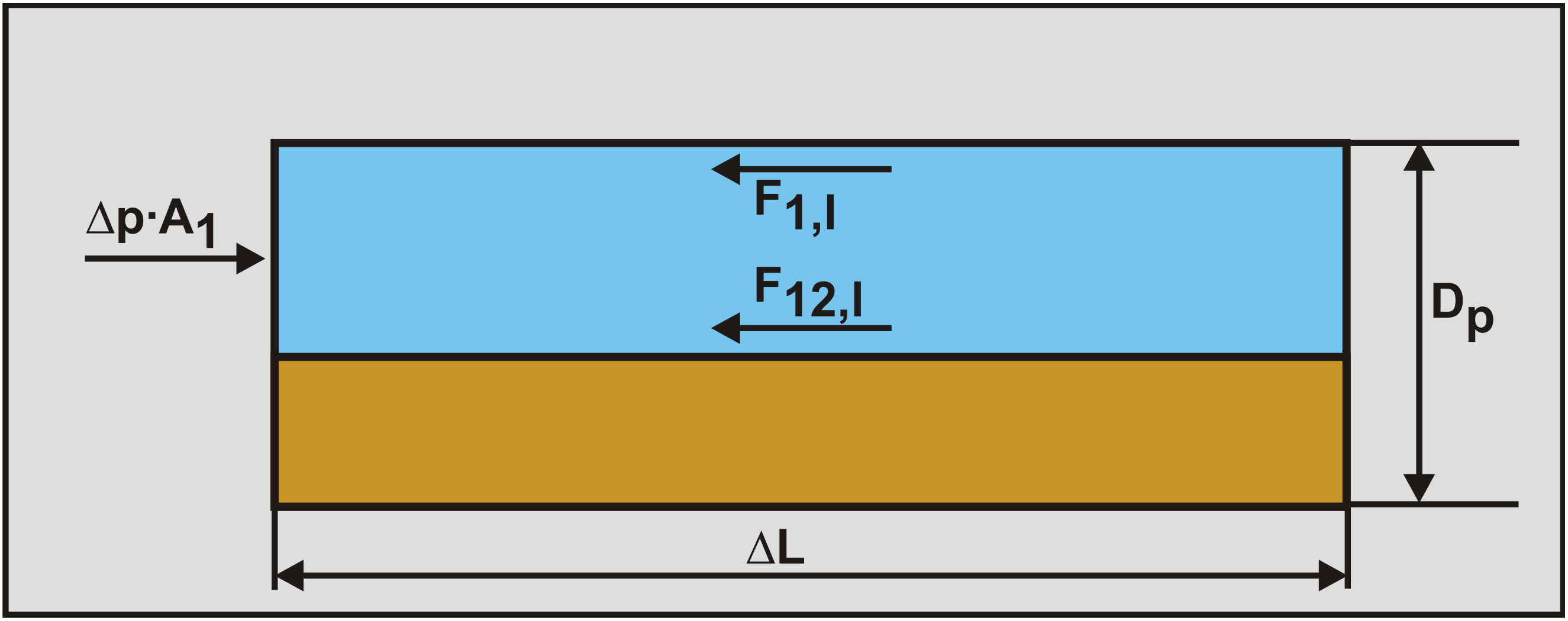
6.20.1.4 The Forces Involved

First the equilibrium of the forces on the liquid above the bed is determined. This is necessary to find the correct hydraulic gradient. The resisting shear force on the pipe wall O₁ above the bed is:

\[\ \mathrm{F}_{\mathrm{1}, \mathrm{l}}=\tau_{\mathrm{1}, \mathrm{l}} \cdot \mathrm{O}_{\mathrm{1}} \cdot \mathrm{\Delta} \mathrm{L}\]

The resisting shear force on the bed surface O₁₂ betweeen the restricted area and the top of the bed is:

\[\ \mathrm{F}_{12,\mathrm{l}}=\tau_{12,\mathrm{l}} \cdot \mathrm{O}_{12} \cdot \Delta \mathrm{L}\]

The pressure Δp on the liquid above the bed is:

\[\ \Delta \mathrm{p}=\Delta \mathrm{p}_{2}=\Delta \mathrm{p}_{1}=\frac{\tau_{1,\mathrm{l}} \cdot \mathrm{O}_{\mathrm{1}} \cdot \Delta \mathrm{L}+\tau_{12,\mathrm{l}} \cdot \mathrm{O}_{12} \cdot \Delta \mathrm{L}}{\mathrm{A}_{1}}=\frac{\mathrm{F}_{1,\mathrm{l}}+\mathrm{F}_{12, \mathrm{l}}}{\mathrm{A}_{1}}\]

The force equilibrium on the liquid above the bed is shown in Figure 6.20-2.

Figure 6.20-2: The forces on the liquid above the bed.

Secondly the equilibrium of forces on the bed is determined as is shown in Figure 6.20-3.

Figure 6.20-3: The forces on the bed.

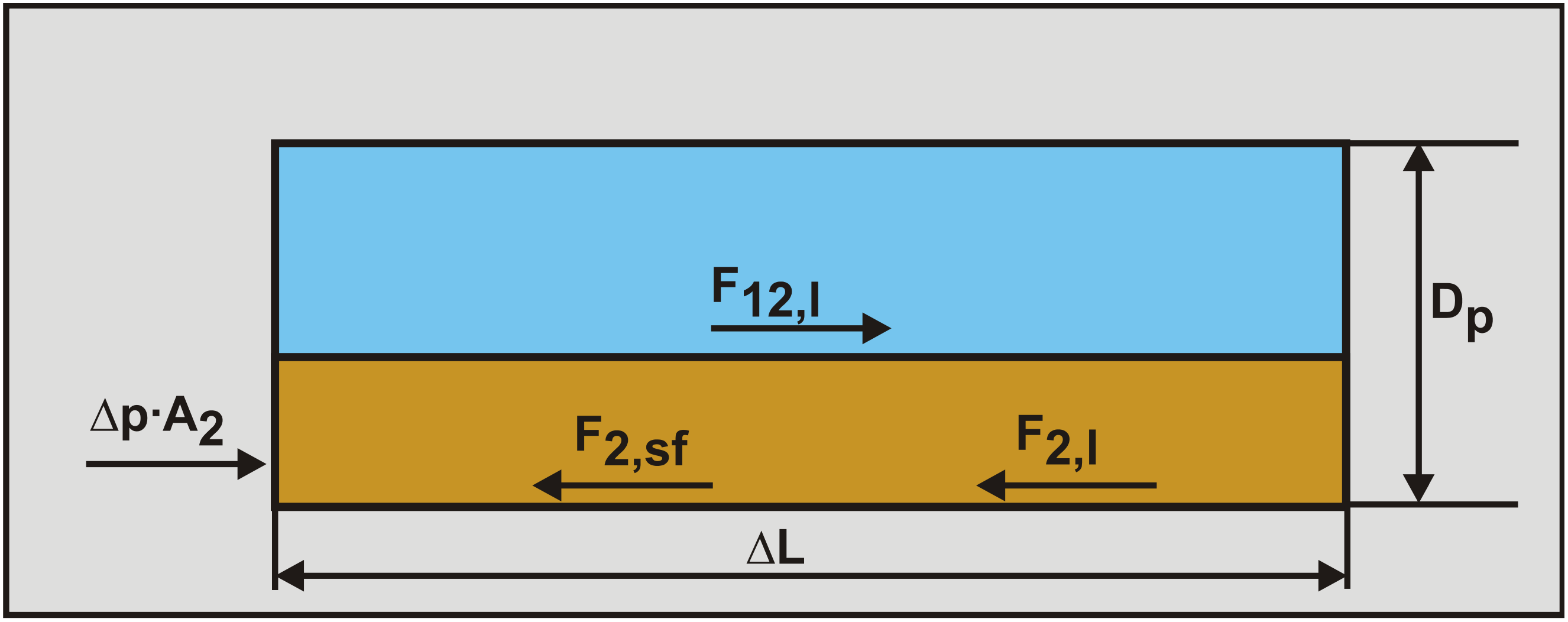
The driving shear force on the bed surface is:

\[\ \mathrm{F}_{\mathrm{1 2}, \mathrm{l}}=\tau_{\mathrm{1 2}, \mathrm{l}} \cdot \mathrm{O}_{\mathrm{1 2}} \cdot \mathrm{\Delta} \mathrm{L}\]

The driving force resulting from the pressure Δp on the bed is:

\[\ \mathrm{F}_{2, \mathrm{p r}}=\Delta \mathrm{p} \cdot \mathrm{A}_{2}\]

The resisting force between the bed and the pipe wall due to sliding friction is:

\[\ \mathrm{F}_{2, \mathrm{sf}}=\tau_{2, \mathrm{sf}} \cdot \mathrm{O}_{2} \cdot \Delta \mathrm{L}\]

The resisting shear force between the liquid in the bed and the pipe wall is:

\[\ \mathrm{F}_{2, \mathrm{l}}=\tau_{2, \mathrm{l}} \cdot \mathrm{O}_{2} \cdot \mathrm{n} \cdot \Delta \mathrm{L}\]

This shear force is multiplied by the porosity n, in order to correct for the fact that the bed consists of a combination of particles and water. There is an equilibrium of forces when:

\[\ \mathrm{F}_{\mathrm{1 2}, \mathrm{l}}+\mathrm{F}_{\mathrm{2}, \mathrm{p r}}=\mathrm{F}_{\mathrm{2}, \mathrm{s f}}+\mathrm{F}_{\mathrm{2}, \mathrm{l}}\]

Below the Limit of Stationary Deposit Velocity, the bed is not sliding and the force F_2,l equals zero. Since the problem is implicit with respect to the velocities v₁ and v₂, it has to be solved with an iteration process.

In the case when the relative concentration C_vr=C_vs/C_vb or C_vr=C_vt/C_vb equals 1, the resistance equals the plug hydraulic gradient, according to:

\[\ \mathrm{i}_{\mathrm{p l u g}}=\mathrm{2} \cdot {\mu}_{\mathrm{s f}} \cdot \mathrm{R}_{\mathrm{s d}} \cdot \mathrm{C}_{\mathrm{v b}}\]

Wilson et al. (1992) defined the maximum Limit of Stationary Deposit Velocity as v_sm.

The graphs in the following chapter are determined for uniform sands, not taking into account grading. In real life there will almost always be grading, resulting in slightly different curves, depending on the grading.

6.20.1.5 Output with the Wilson et al. (1992) Hydrostatic Stress Approach

Figure 6.20-4: The hydraulic gradient i_m versus the line speed v_ls, C_vr=C_vs/C_vb.

Figure 6.20-5: The normalized hydraulic gradient i_m/i_plug versus the relative line speed v_r, C_vr=C_vs/C_vb.

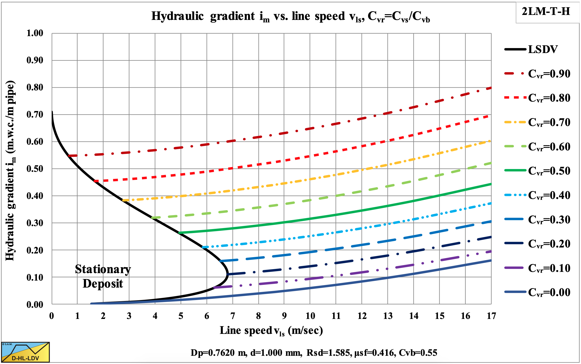
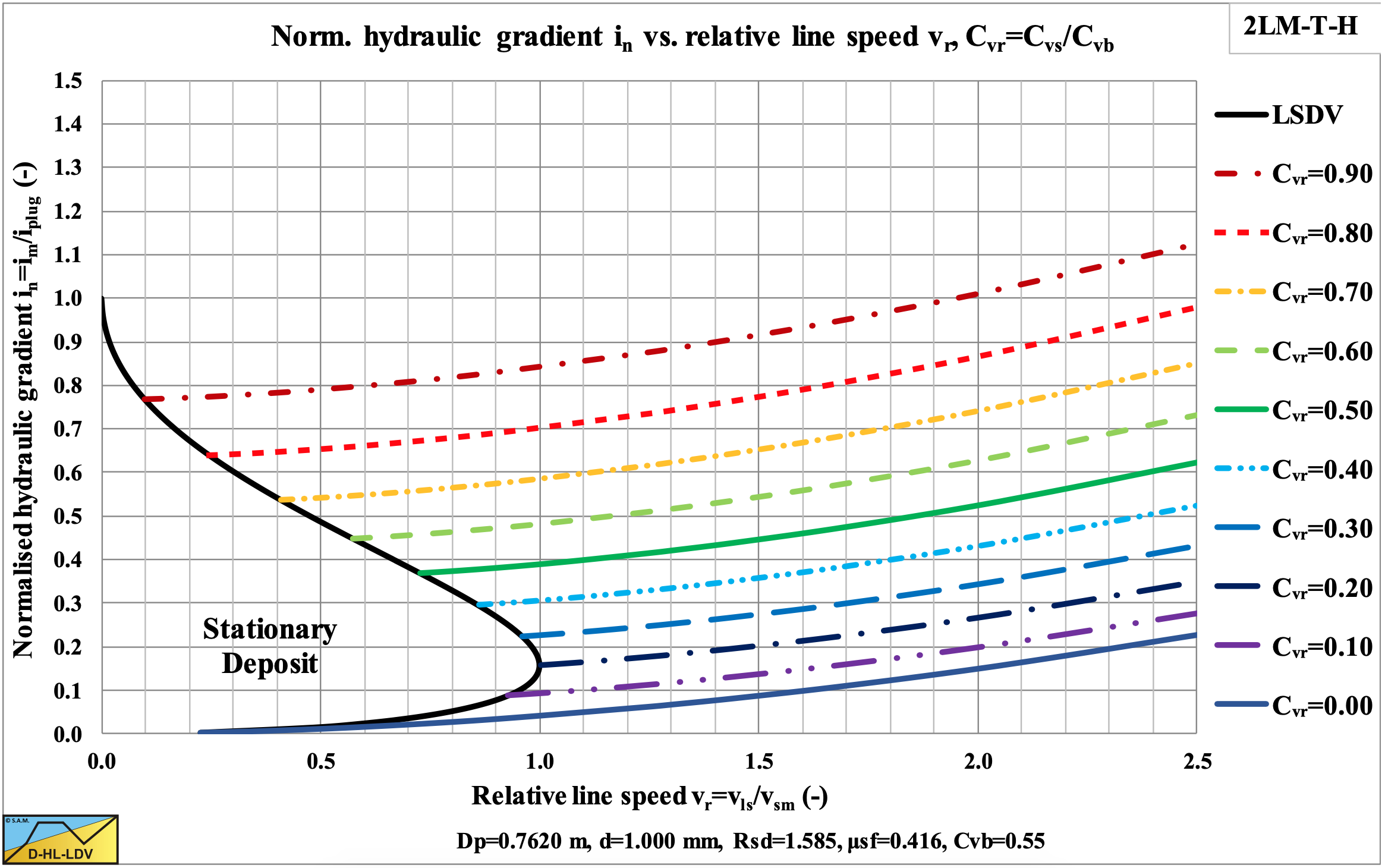
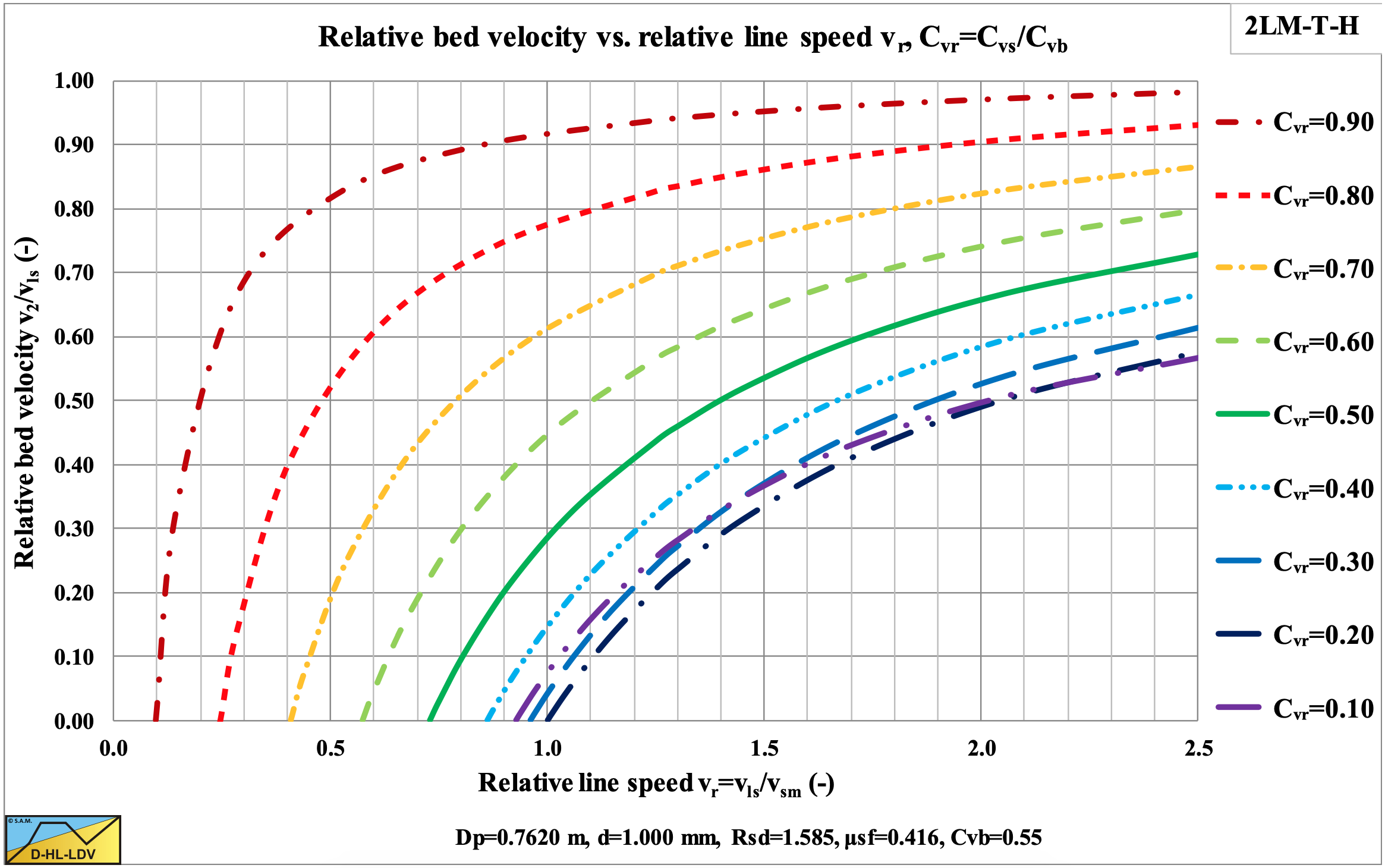
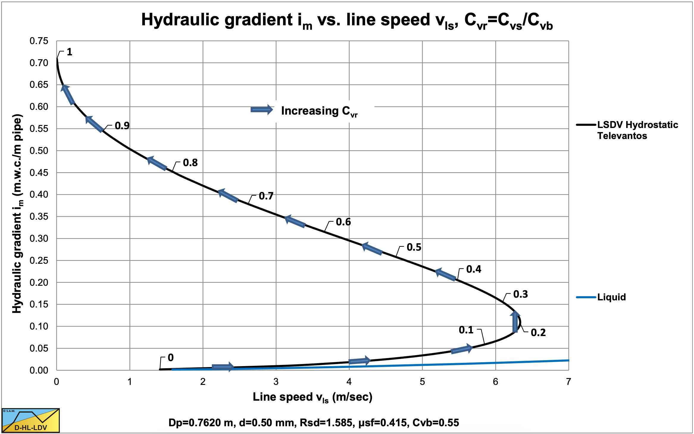
The direct outputs of the model are the hydraulic gradient and the bed velocity as shown in Figure 6.20-4, Figure 6.20-5 and Figure 6.20-6. Based on the bed velocity the delivered volumetric concentration C_vt and the slip velocity v_sl can be determined as is shown in Figure 6.20-7 and Figure 6.20-8. In Figure 6.20-5 the axis are made dimensionless (normalized) by dividing the hydraulic gradient by the plug hydraulic gradient and dividing the line speed v_ls by the maximum Limit of Stationary Deposit Velocity v_sm. The relative bed velocity increases with increasing relative spatial volumetric concentration and even becomes 1 for a relative spatial concentration of 1, the bed concentration. The transport or delivered volumetric concentration also increases with increasing relative spatial volumetric concentration, but also with an increasing line speed.

Figure 6.20-6: The relative bed velocity v₂/v_sl versus the relative line speed v_r, C_vr=C_vs/C_vb.

Figure 6.20-7: The relative volumetric transport concentration C_vr=C_vs/C_vb vs. the relative line speed v_r.

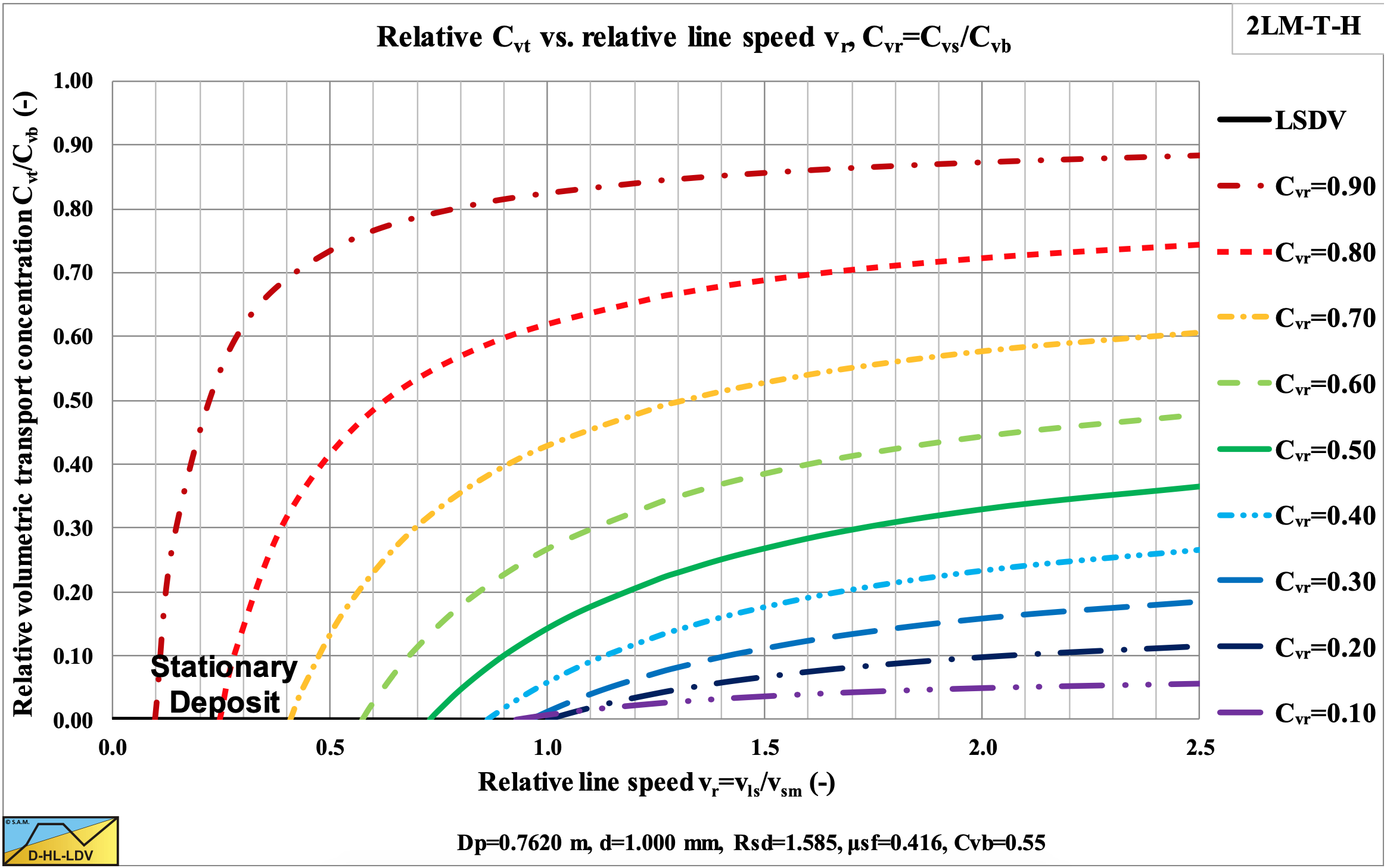
Once the delivered volumetric concentration is known, points with equal delivered concentration can be connected and hydraulic gradient curves with constant delivered volumetric concentration can be constructed as is shown in Figure 6.20-9 and Figure 6.20-10. It should be mentioned that these curves do not intersect with the limit of stationary deposit velocity curve, since there the bed has no velocity, so the delivered concentration is zero. The curves with small delivered concentrations follow the Limit of Stationary Deposit Velocity curve at the upper side. Figure 6.20-8 shows that the slip velocity decreases with an increasing spatial volumetric concentration and even goes to zero if the relative spatial concentration goes to 1, the bed concentration.

Figure 6.20-8: The relative slip velocity v_sl/v_ls versus the relative line speed v_r, C_vr=C_vs/C_vb.

Figure 6.20-9: The hydraulic gradient i_m versus the line speed v_ls, C_vr=C_vt/C_vb.

Figure 6.20-10: The normalized hydraulic gradient i_m/i_plug versus the relative line speed v_r, C_vr=C_vt/C_vb.

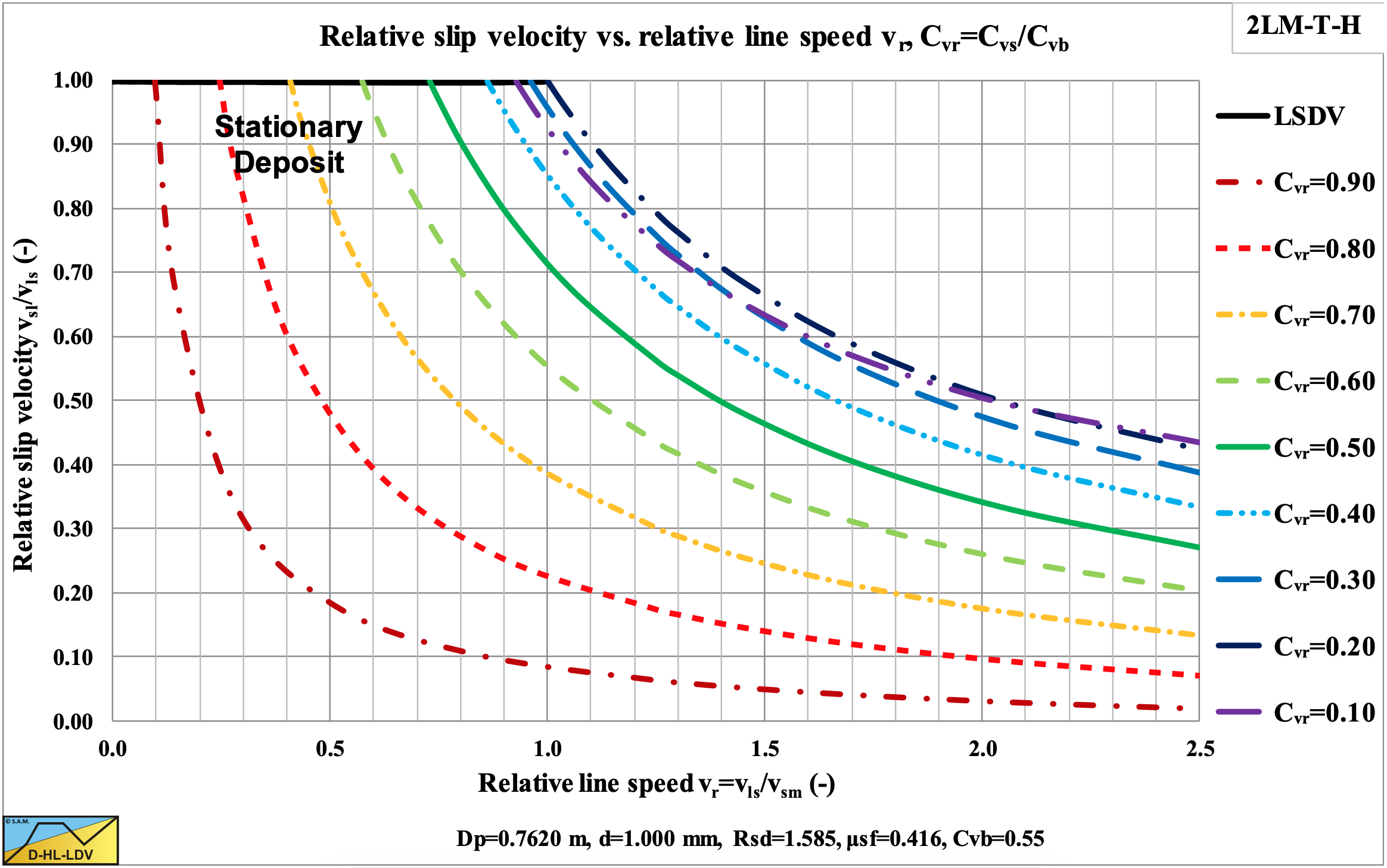
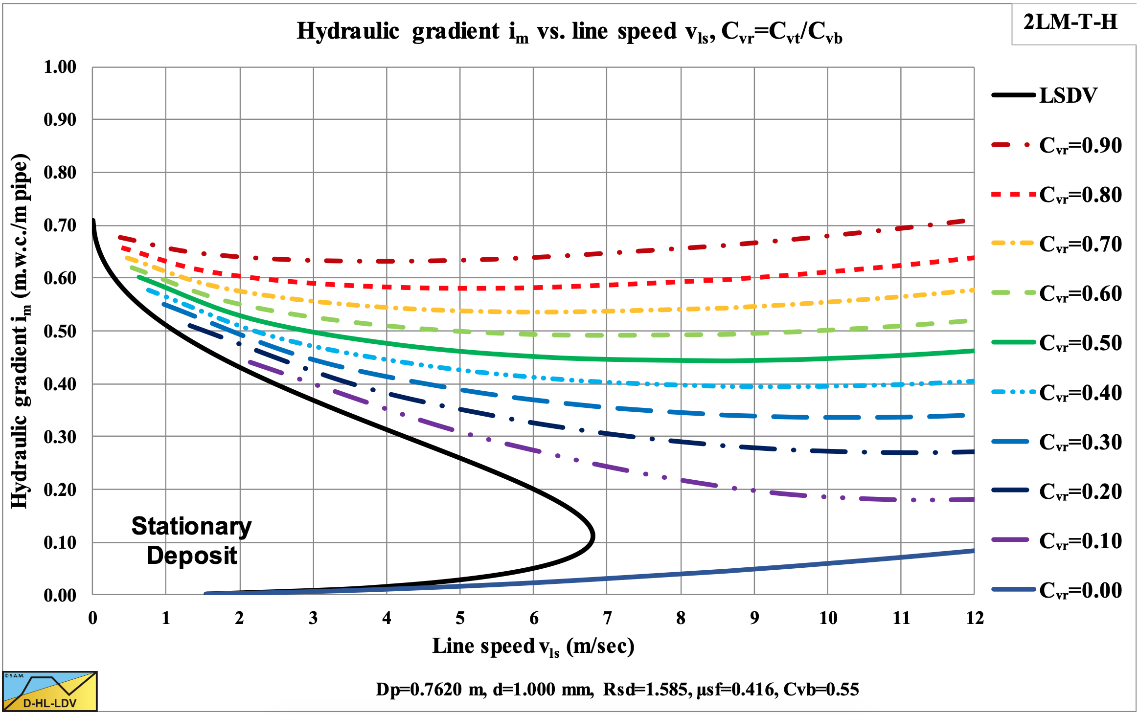
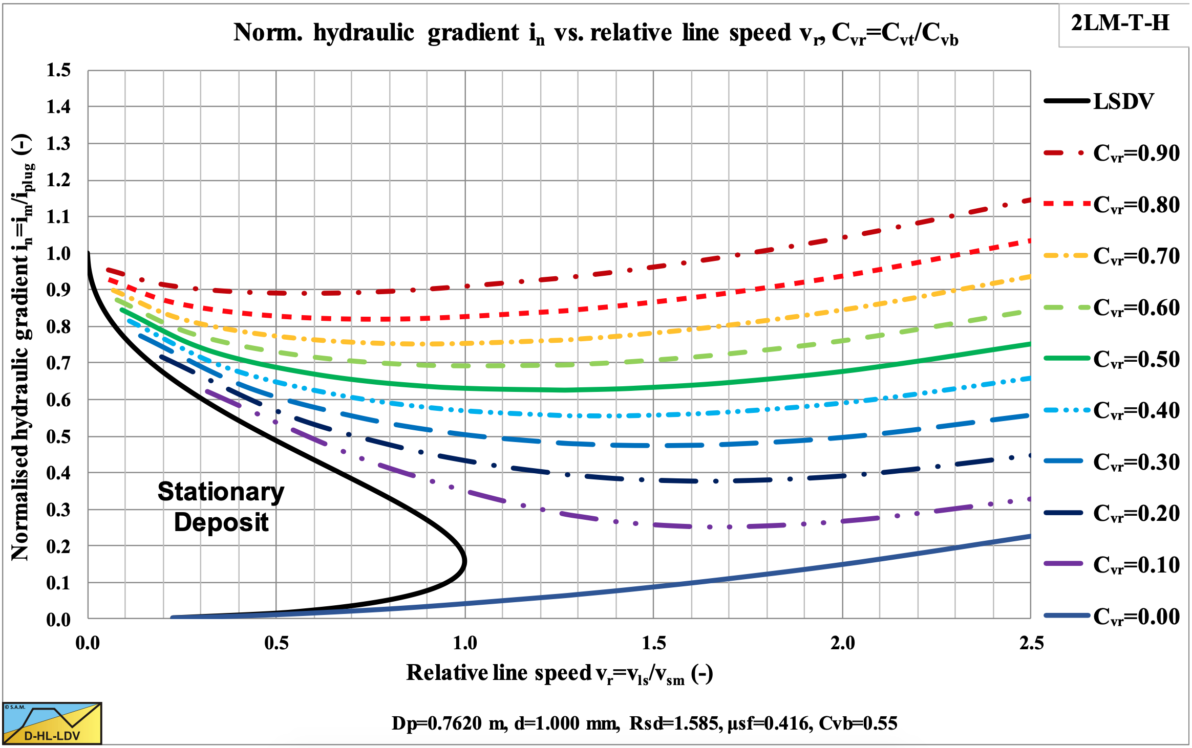
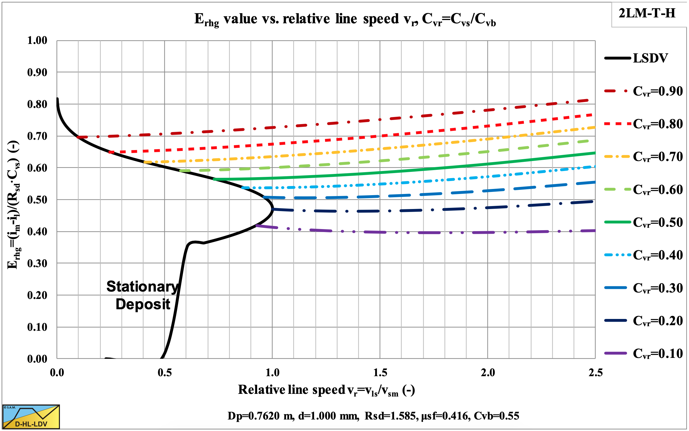
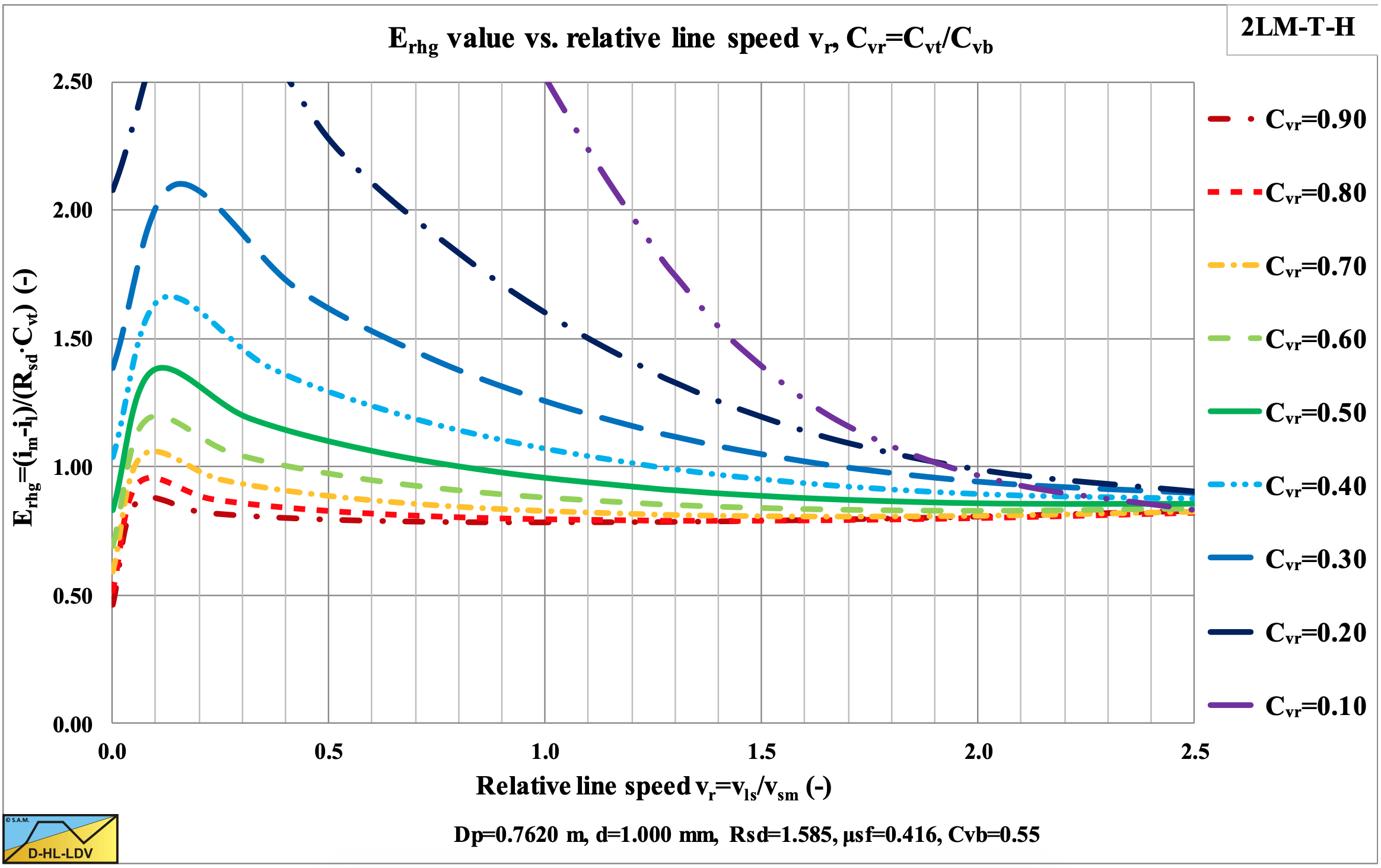
Figure 6.20-11 and Figure 6.20-12 show the relative excess hydraulic gradient curves for constant spatial volumetric concentration curves and for constant delivered volumetric concentration curves. The constant spatial volumetric concentration curves are almost horizontal, but have a higher value for a higher relative spatial volumetric concentration, due to the hydrostatic pressure approach for the normal stresses between the bed and the pipe wall. For low relative spatial volumetric concentrations, the relative excess hydraulic gradient has a value close to the sliding friction coefficient μ_sf. A relative spatial volumetric concentration of 1 results in a relative excess hydraulic gradient of about 2 times the sliding friction coefficient.

Figure 6.20-11: The relative excess hydraulic gradient E_rhg versus the relative line speed v_r, C_vr=C_vs/C_vb.

Figure 6.20-12: The relative excess hydraulic gradient E_rhg versus the relative line speed v_r, C_vr=C_vt/C_vb.

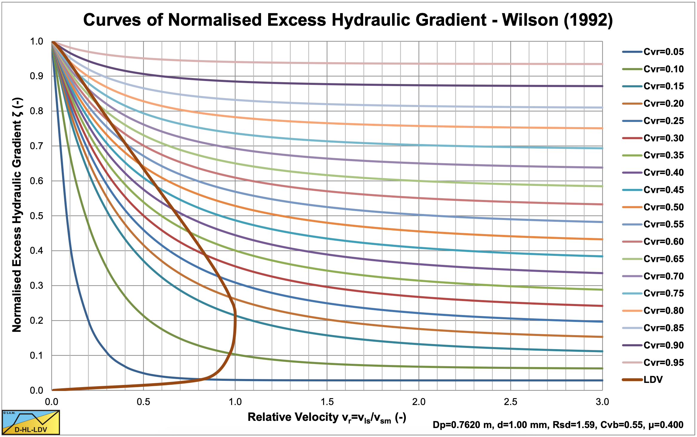
Wilson et al. (1992) often show the excess hydraulic gradient divided (normalized) by the plug hydraulic gradient in their graphs, like in Figure 6.20-13. Their fit functions are also based on this type of graph.

Figure 6.20-13: The normalized excess hydraulic gradient (i_m-i_l)/i_plug versus the relative line speed v_r, C_vr=C_vt/C_vb.

6.20.1.6 The Fit Functions of Wilson et al. (1992)

Wilson et al. (1992) published the sliding bed model as a nomograph, using a set of parameters (μ_sf=0.4, C_vb=0.6 and a factor α=2.75 for the friction factor on top of the bed). The nomograph and the set of fit function for the normalized excess hydraulic gradient are based on constant volumetric transport concentration curves.

The normalized excess hydraulic gradient is defined as the mixture hydraulic gradient minus the liquid hydraulic gradient divided by the plug hydraulic gradient:

\[\ \zeta=\frac{\mathrm{i}_{\mathrm{m}}-\mathrm{i}_{\mathrm{l}}}{\mathrm{i}_{\mathrm{p l u g}}}=\frac{\mathrm{i}_{\mathrm{m}}-\mathrm{i}_{\mathrm{l}}}{\mathrm{2} \cdot \boldsymbol{\mu}_{\mathrm{s f}} \cdot \mathrm{R}_{\mathrm{s d}} \cdot \mathrm{C}_{\mathrm{v} \mathrm{b}}}\]

The relative line speed is the ratio between the line speed and the maximum Limit of Stationary Deposit Velocity:

\[\ \mathrm{v}_{\mathrm{r}}=\frac{\mathrm{v}_{\mathrm{l s}}}{\mathrm{v}_{\mathrm{s m}}}\]

The relative volumetric transport concentration C_vr is:

\[\ \mathrm{C}_{\mathrm{v r}}=\frac{\mathrm{C}_{\mathrm{v t}}}{\mathrm{C}_{\mathrm{v b}}}\]

The maximum Limit of Stationary Deposit Velocity (LSDV) v_sm can be estimated by (Matousek (2004)), with d in mm and D_p in m:

\[\ \mathrm{v}_{\mathrm{s m}}=\frac{\mathrm{8.8 } \cdot\left(\frac{\mu_{\mathrm{sf}} \cdot \mathrm{R}_{\mathrm{sd}}}{\mathrm{0 . 6 6}}\right)^{\mathrm{0 . 5 5}} \cdot \mathrm{D}_{\mathrm{p}}^{\mathrm{0 . 7}} \cdot \mathrm{d}^{\mathrm{1 . 7 5}}}{\mathrm{d}^{2}+\mathrm{0 . 1 1 \cdot D _ { \mathrm { p } } ^ { \mathrm { 0 . 7 } }}} \quad\text{ and }\quad \mathrm{F}_{\mathrm{L}}=\frac{\mathrm{v}_{\mathrm{s m}}}{\sqrt{\mathrm{2 \cdot \mathrm { g } \cdot \mathrm { R } _ { \mathrm { s d } } \cdot \mathrm { D } _ { \mathrm { p } }}}}\]

Figure 6.20-14: The Durand Froude number F_L based on v_sm for sands and gravels.

Figure 6.20-14 shows the Durand Froude number F_L for a number of pipe diameters as a function of the particle diameter. The figure also shows the Durand Froude number of the intersection point of the (slightly modified) heterogeneous model with the sliding bed curve (Transition FB-He). If this intersection point is below the LSDV, a sliding bed will never occur, if it is above the LSDV a sliding bed will occur. The figure shows the particle diameter where the sliding bed will occur for each pipe diameter. Other heterogeneous models may give slightly different values.

In the smallest (D_p=1 inch and 2 inch) pipe a sliding bed will always occur. A pipe diameter of D_p=0.1016 m gives d=0.49 mm, D_p=0.1524 m gives d=0.78 mm, D_p=0.254 m gives d=1.3 mm, D_p=0.5 m gives d=2.65 mm, D_p=0.762 m gives d=3.8 mm. In the largest (D_p=1 m) pipe a sliding bed will occur for particles larger than about d=4.5 mm. The conclusion is, that one cannot just scale head losses, without knowing the flow regimes occurring. The demi-McDonald is shown in Figure 6.20-37 with an example.

The volumetric transport concentration at this maximum Limit of Stationary Deposit Velocity can be estimated by, with d in mm and D_p in m (for C_rm in the range 0.05-0.66):

\[\ \mathrm{C}_{\mathrm{rm}}=\mathrm{C}_{\mathrm{vr}, \mathrm{max}}=\mathrm{0.16} \cdot \mathrm{D}_{\mathrm{p}}^{0.40} \cdot \mathrm{d}^{-0.84} \cdot\left(\frac{\mathrm{R}_{\mathrm{sd}}}{1.65}\right)^{-0.17}\]

Figure 6.20-15: The maximum relative solids concentration versus the particle diameter.

For other volumetric transport concentrations, the Limit of Stationary Deposit Velocity v_s can be estimated by:

\[\ \begin{array}{left}\frac{\mathrm{v}_{\mathrm{s}}}{\mathrm{v}_{\mathrm{sm}}}=\mathrm{6.75} \cdot \mathrm{C}_{\mathrm{vr}}^{\alpha} \cdot\left(1-\mathrm{C}_{\mathrm{vr}}^{\alpha}\right)^{2} \quad\text{ if }\quad \mathrm{C}_{\mathrm{vr}, \max } \leq \mathrm{0.33}\\
\frac{\mathrm{v}_{\mathrm{s}}}{\mathrm{v}_{\mathrm{sm}}}=\mathrm{6.75} \cdot\left(\mathrm{1}-\mathrm{C}_{\mathrm{vr}}\right)^{2 \cdot \beta} \cdot\left(1-\left(1-\mathrm{C}_{\mathrm{vr}}\right)^{\beta}\right) \quad\text{ if }\quad \mathrm{C}_{\mathrm{vr}, \max }>0.33\\
\text{ With: } \quad \alpha=\frac{\ln (0.333)}{\ln \left(\mathrm{C}_{\mathrm{vr}, \max }\right)} \quad\text{ and }\quad \beta=\frac{\ln (0.666)}{\ln \left(1-\mathrm{C}_{\mathrm{vr}, \max }\right)}\end{array}\]

The asymptotic normalized excess hydraulic gradient for very high line speeds can be determined by:

\[\ \zeta_{\infty}=\mathrm{0 . 5} \cdot \mathrm{C}_{\mathrm{vr}} \cdot\left(1+\mathrm{C}_{\mathrm{vr}}^{0.66}\right)\]

For lower line speeds the normalized excess hydraulic gradient can now be determined by:

\[\ \begin{array}{left}\zeta=\zeta_{\infty}+\left(1-\zeta_{\infty}\right) \cdot\left(1+\mathrm{v}_{\mathrm{r}}\right)^{-\mathrm{q}}\\
\mathrm{q}=3.6-\mathrm{5} .2 \cdot \mathrm{C}_{\mathrm{vr}} \cdot\left(1-\mathrm{C}_{\mathrm{vr}}\right) \quad\text{ if }\quad \mathrm{C}_{\mathrm{vr}} \geq \mathrm{C}_{\mathrm{vr}, \max }\end{array}\]

or

\[\ \mathrm{q}=\left(3.6-5.2 \cdot \mathrm{C}_{\mathrm{vr}, \max } \cdot\left(1-\mathrm{C}_{\mathrm{vr}, \max }\right)\right) \cdot \frac{\mathrm{C}_{\mathrm{vr}, \max }}{\mathrm{C}_{\mathrm{vr}}} \quad\text{ if }\quad \mathrm{C}_{\mathrm{vr}}<\mathrm{C}_{\mathrm{vr}, \mathrm{max}}\]

Figure 6.20-16: The relative deposit velocity versus the relative concentration.

Figure 6.20-14 shows the maximum Durand Froude number as a function of the particle diameter (in mm) and the pipe diameter (in m). Figure 6.20-15 shows how the concentration where the maximum LSDV occurs depends on the particle diameter (in mm) and the pipe diameter (in m). Figure 6.20-16 shows how the LSDV depends on the relative concentration and the concentration where the maximum LSDV occurs. Figure 6.20-17 shows a resulting LSDV curve.

Later a shear layer or sheet flow layer was incorporated. If the sharp interface between a bed and the carrier liquid above the bed is replaced by a shear layer, the driving force at the interface is no longer dependent on the roughness of the bed. Therefore the particle size does not influence the maximum LSDV. The Durand Froude number can be determined with the following equation in this case:

\[\ \mathrm{F}_{\mathrm{L}}=\frac{\mathrm{v}_{\mathrm{s m}}}{\sqrt{\mathrm{2} \cdot \mathrm{g} \cdot \mathrm{R}_{\mathrm{s d}} \cdot \mathrm{D}_{\mathrm{p}}}}=\left(\frac{\mathrm{0.} \mathrm{0} \mathrm{1} \mathrm{8}}{\lambda_{\mathrm{l}}}\right)^{0 . \mathrm{1 3}}\]

The smaller of the two LSDV approximations should be chosen. The above equation is derived fro a specific bed concentration and sliding friction coefficient. Other conditions may give a slightly different equation.

Figure 6.20-17: The LSDV curve.

With these equations, Figure 6.20-18 is reconstructed.

Figure 6.20-18: The fit functions of Wilson et al. (1992).

Of course the curves cannot exist inside the stationary bed region. However here the curves are shown as given by Wilson. This comment is also valid for the next figure.

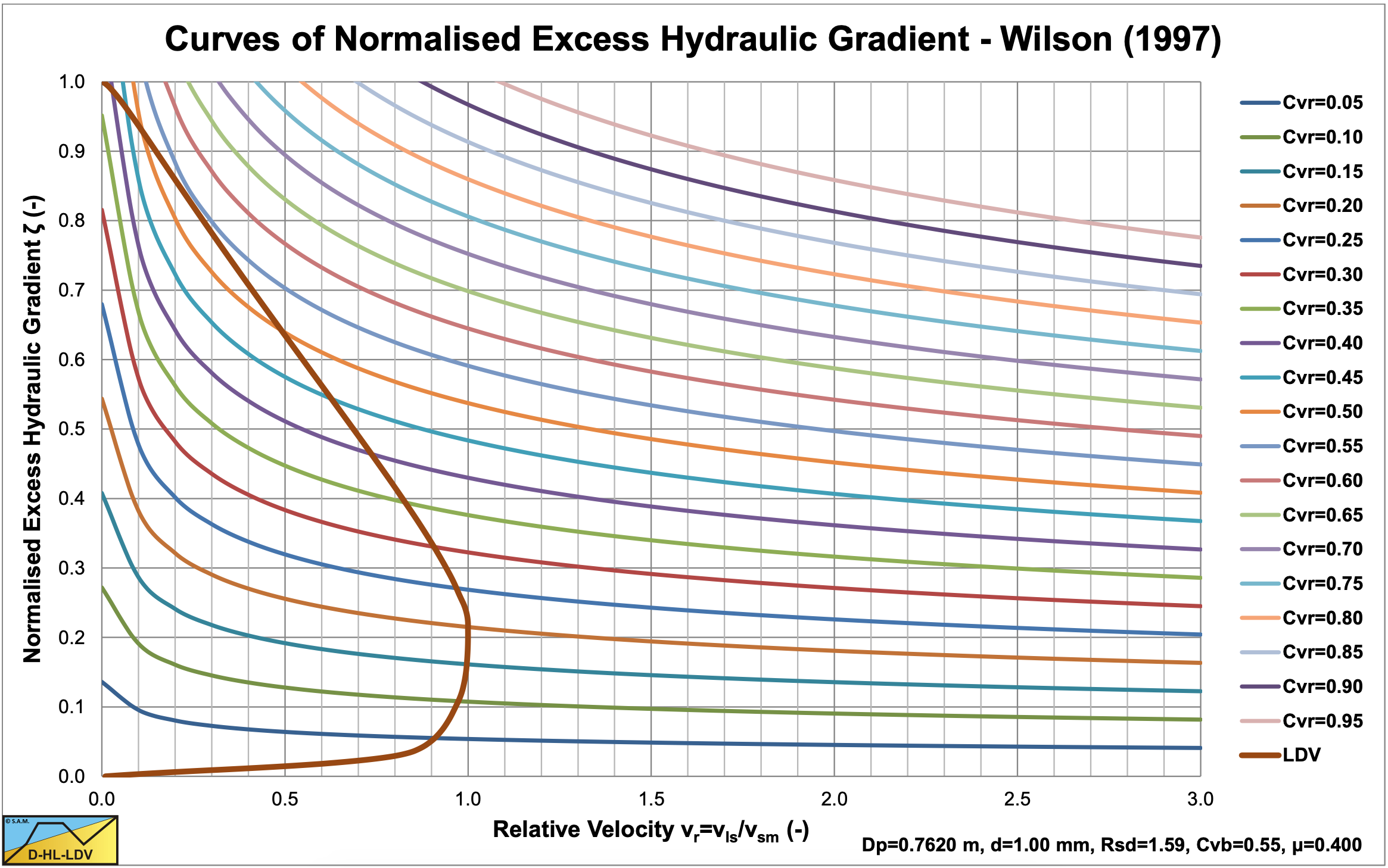
6.20.1.7 The Fit Functions of Wilson et al. (1997)

The relative excess hydraulic gradient can be approximated by (for a sliding friction coefficient of 0.4 and 0.44):

\[\ \begin{array}{left} \mathrm{E}_{\mathrm{r h g}}=\frac{\mathrm{i}_{\mathrm{m}}-\mathrm{i}_{\mathrm{l}}}{\mathrm{R}_{\mathrm{s} \mathrm{d}} \cdot \mathrm{C}_{\mathrm{v} \mathrm{t}}}=\left(\frac{\mathrm{0 . 5 5} \cdot \mathrm{v}_{\mathrm{s m}}}{\mathrm{v}_{\mathrm{l s}}}\right)^{0.25}=\mathrm{0 . 8 6 1} \cdot\left(\frac{\mathrm{v}_{\mathrm{s m}}}{\mathrm{v}_{\mathrm{l s}}}\right)^{0.25}=\mathrm{2} \cdot \mu_{\mathrm{s f}} \cdot\left(\frac{\mathrm{4} \cdot \mathrm{v}_{\mathrm{s m}}}{\mathrm{3} \cdot \mathrm{v}_{\mathrm{l s}}}\right)^{0.25} \quad\text{ for }\mu_{\mathrm{s f}}=\mathrm{0 . 4 0}\\
\mathrm{E}_{\mathrm{r h g}}=\frac{\mathrm{i}_{\mathrm{m}}-\mathrm{i}_{\mathrm{l}}}{\mathrm{R}_{\mathrm{s d}} \cdot \mathrm{C}_{\mathrm{v t}}}=\left(\frac{\mathrm{0 . 5 5 \cdot v}_{\mathrm{s m}}}{\mathrm{v}_{\mathrm{l s}}}\right)^{0.25}=\mathrm{0 . 8 6 1} \cdot\left(\frac{\mathrm{v}_{\mathrm{s m}}}{\mathrm{v}_{\mathrm{l s}}}\right)^{0.25}=\mathrm{2} \cdot \mu_{\mathrm{s f}} \cdot\left(\frac{\mathrm{v}_{\mathrm{s m}}}{\mathrm{v}_{\mathrm{l s}}}\right)^{0.25} \quad\text{ for }\mu_{\mathrm{sf}}=\mathrm{0 . 4 4}\end{array}\]

In the case where the line speed equals the maximum Limit of Stationary Deposit Velocity v_sm, this gives:

\[\ \mathrm{E}_{\mathrm{rhg}}=\frac{\mathrm{i}_{\mathrm{m}}-\mathrm{i}_{\mathrm{l}}}{\mathrm{R}_{\mathrm{sd}} \cdot \mathrm{C}_{\mathrm{vt}}}=2 \cdot \mu_{\mathrm{sf}} \cdot\left(\frac{4}{3}\right)^{0.25} \quad\text{ or }\quad \mathrm{E}_{\mathrm{rhg}}=\frac{\mathrm{i}_{\mathrm{m}}-\mathrm{i}_{\mathrm{l}}}{\mathrm{R}_{\mathrm{sd}} \cdot \mathrm{C}_{\mathrm{vt}}}=2 \cdot \mu_{\mathrm{sf}}\]

This gives for the normalized excess hydraulic gradient at this line speed:

\[\ \zeta=\frac{\mathrm{i}_{\mathrm{m}}-\mathrm{i}_{\mathrm{l}}}{\mathrm{i}_{\mathrm{plug}}}=\frac{\mathrm{2} \cdot \mu_{\mathrm{s f}} \cdot \mathrm{R}_{\mathrm{s d}} \cdot \mathrm{C}_{\mathrm{v t}}}{\mathrm{2} \cdot \mathrm{\mu}_{\mathrm{s f}} \cdot \mathrm{R}_{\mathrm{s d}} \cdot \mathrm{C}_{\mathrm{v} \mathrm{b}}}=\frac{\mathrm{C}_{\mathrm{v t}}}{\mathrm{C}_{\mathrm{v b}}} \cdot\left(\frac{4}{\mathrm{3}}\right)^{\mathrm{0 . 2 5}} \quad\text{ or }\quad \zeta=\frac{\mathrm{i}_{\mathrm{m}}-\mathrm{i}_{\mathrm{l}}}{\mathrm{i}_{\mathrm{p l u g}}}=\frac{\mathrm{C}_{\mathrm{v} \mathrm{t}}}{\mathrm{C}_{\mathrm{v} \mathrm{b}}}\]

Figure 6.20-19 shows the resulting normalized excess hydraulic gradient curves.

Figure 6.20-19: The fit functions of Wilson et al. (1997).

6.20.1.8 The Stratification Ratio

The Wilson et al. (1997) model is based on a 100% stationary or sliding bed giving 100% stratification. However at a certain velocity of the liquid above the bed erosion may occur, related to the Shields parameter as described in chapter 5. It is also possible that a shear layer or sheet flow occurs at the top of the bed. Erosion will reduce the bed thickness while a shear layer or sheet flow will influence the Moody friction coefficient at the top of the bed. Whatever the mechanism may be, the bed will dissolve with increasing line speed and transit to (pseudo) homogeneous flow at (very) high line speeds. In order to take this into account, Wilson et al. (1997) defined a stratification ratio, being the amount of particles in the bed (in contact) divided by the total amount of particles in a cross section of the pipe.

\[\ \mathrm{R}=\frac{\mathrm{C}_{\mathrm{vc}}}{\mathrm{C}_{\mathrm{v s}}}\]

If all the available particles are in the bed the stratification ratio is 1 or 100%. If all the available particles are in suspension the stratification ratio is 0 or 0%. The amount of particles in suspension, being part of the homogeneous, equivalent liquid model, flow equals 1 minus the stratification ratio. To determine the total hydraulic gradient Wilson et al. (1997) adds the stratification ratio times the bed resistance and 1 minus the stratification ratio times the ELM resistance according to:

\[\ \mathrm{i}_{\mathrm{m}}=\mathrm{R} \cdot \mathrm{i}_{\mathrm{b e d}}+(\mathrm{1}-\mathrm{R}) \cdot \mathrm{i}_{\mathrm{h o m}}\]

Basically this means that the superposition principle is applied on a mix of the sliding bed regime and the homogeneous regime. This implies that the behavior of both processes is linear, which does not have to be the case. However, by determining the formulation of the stratification ratio experimentally, resulting in an empirical equation, this will correct itself. This empirical equation is determined based on the hydraulic gradient and not based on the real stratification ratio.

6.20.1.9 Suspension in the Upper Layer

The basic Wilson et al. (1992) two layer model considers a fixed or sliding bed with water above the bed. So we have a bed layer and a water layer. Wilson et al. (1990) defined a threshold velocity at which particles start suspending. This threshold velocity is defined as:

\[\ \mathrm{v}_{\mathrm{u}}=\mathrm{v}_{\mathrm{t}} \cdot \sqrt{\frac{\mathrm{8}}{\lambda_{\mathrm{l}}}}{ \cdot \mathrm{e}^{\frac{45 \cdot \mathrm{d}}{\mathrm{D}_{\mathrm{p}}}}} \quad\text{ or }\quad \mathrm{u}_{*}=\sqrt{\frac{\lambda_{\mathrm{l}}}{\mathrm{8}}}{ \cdot \mathrm{v}_{\mathrm{u}}}=\mathrm{v}_{\mathrm{t}} \cdot \mathrm{e}^{\frac{4 \mathrm{5} \cdot \mathrm{d}}{\mathrm{D_p}}}\]

\[\ \mathrm{R}=\left(\frac{\mathrm{v}_{\mathrm{u}}}{\mathrm{v}_{\mathrm{ls}}}\right)^{\mathrm{M}}\]

So when the line speed v_ls equals the threshold velocity v_u, the stratification ratio R equals 1, meaning that 100% of the particles is in the bed. As the line speed increases, the stratification ratio decreases. The power M has a value of 1.7 for very narrow graded sands or gravels, uniform sands or gravels. The more graded a sand or gravel, the smaller the power M with a minimum of 0.25. This approach forms the basis of the heterogeneous model of Wilson et al. (1992). The amount of solids in suspension is now 1-C_vc/C_vs=(1-R).

By determining the amount of solids in suspension and adjusting the fluid density and viscosity and the amount of solids in the bed, the two layer model can be applied for small particles. The Thomas (1965) equation can be used to adjust the viscosity of the liquid/solid mixture. This explains decrease of the LSDV with decreasing particle diameter for particles smaller than about d=0.7 mm. It also explains for the increase of the spatial concentration where the maximum LSDV occurs with decreasing particle diameter. The delivered concentration is in this case C_vt=(1-R)·C_vs. For other solids densities this behavior may be different, since large particles probably have a different influence on the viscosity.

6.20.1.10 Conclusions & Discussion

The Wilson et al. (1992) model forms a solid base for 2 layer and 3 layer models. The model is based on the force equilibrium on the bed and is capable of determining the Limit of Stationary Deposit Velocity curve for the start of sliding of the bed. The model also gives the bed velocity for line speeds above the Limit of Stationary Deposit Velocity. Although the model is based on constant spatial volumetric concentration curves, based on the bed velocity the delivered volumetric concentration can be determined. Connecting points with constant delivered volumetric concentration, enables to construct constant delivered volumetric concentration curves as used in practice. The model however still has a number of shortcomings. First of all, the Darcy-Weisbach friction factor on the bed is assumed to be constant, not depending on the velocity above the bed (Wilson uses a factor 2 or 2.75). Since above a certain line speed the top layer of the bed will be sheet flow, the Darcy-Weisbach friction factor will increase with increasing line speed. Sheet flow also implies higher velocities of the particles in the sheet flow layer, resulting in higher delivered volumetric concentrations. The model however assumes a solid sliding bed without any particles above the bed, either in suspension or in a sheet flow layer. A second shortcoming is the hydrostatic normal stress between the bed and the wall. This assumption in the model also neglects the presence of particles in suspension or in a sheet flow layer apart from the fact that this assumption is questionable in the first place for beds occupying more than 50% of the pipe. The hydrostatic approach implies an upwards component of the normal stress between the bed and the pipe wall in this case, which normally will not occur.

With regard to the fit functions of Wilson et al. (1992) and (1997), in both cases the fit lines intersect with the Limit of Stationary Deposit Velocity curve, which is not physically possible, since the delivered volumetric concentration is zero on these lines. At line speeds much higher than the Limit of Stationary Deposit Velocity, the fit curves may however be correct.

Since Wilson et al. (1992) and (1997) developed the model in a time period without sophisticated computers and software as we have today, it must have been a tedious job to create his graphs. Nowadays a relatively simple Excel sheet can do the job, resulting in the graphs as shown in this chapter.

Later researchers improved the model, like Doron et al. (1987) a two layer model, Doron & Barnea (1993) a three layer model and Matousek (1997) two and three layer models.

6.20.2 The Wilson-GIW (1992) Model for Heterogeneous Transport

6.20.2.1 The Full Model

Assuming that 50% of the solids is moving in the bed by granular contact at a line speed of v₅₀, and assuming a friction coefficient μ_sf between the particles and the pipe wall, the friction force in a pipe with length ΔL is:

\[\ \mathrm{F}_{\mathrm{s f}}=\frac{\mu_{\mathrm{s f}}}{2} \cdot \mathrm{A}_{\mathrm{p}} \cdot \Delta \mathrm{L} \cdot \mathrm{C}_{\mathrm{v}} \cdot\left(\rho_{\mathrm{s}}-\rho_{\mathrm{l}}\right) \cdot \mathrm{g}\]

This gives an excess pressure due to the solids of:

\[\ \Delta \mathrm{p}_{\mathrm{m}}-\Delta \mathrm{p}_{\mathrm{l}}=\frac{\mathrm{F}_{\mathrm{s f}}}{\mathrm{A}_{\mathrm{p}}}=\frac{\mu_{\mathrm{s f}}}{2} \cdot \Delta \mathrm{L} \cdot \mathrm{C}_{\mathrm{v}} \cdot\left(\rho_{\mathrm{s}}-\rho_{\mathrm{l}}\right) \cdot \mathrm{g}\]

In terms of the hydraulic gradient this can be written as:

\[\ \mathrm{i}_{\mathrm{m}}-\mathrm{i}_{\mathrm{l}}=\frac{\Delta \mathrm{p}_{\mathrm{m}}-\Delta \mathrm{p}_{\mathrm{l}}}{\rho_{\mathrm{l}} \cdot \mathrm{g} \cdot \Delta \mathrm{L}}=\frac{\mu_{\mathrm{s f}}}{\mathrm{2}} \cdot \mathrm{C}_{\mathrm{v}} \cdot \frac{\left(\rho_{\mathrm{s}}-\rho_{\mathrm{l}}\right)}{\rho_{\mathrm{l}}}=\frac{\mu_{\mathrm{s f}}}{\mathrm{2}} \cdot \mathrm{C}_{\mathrm{v}} \cdot \mathrm{R}_{\mathrm{s d}}\]

Wilson (1997) has defined a stratification ratio or relative solids effect, which tells which fraction of the particles, is in suspension and which part is in the fixed or moving bed, supported by granular contact. Wilson (1997) gives the following general equation for the head losses in hydraulic transport, where μ_sf equals the friction factor of a sliding bed, which he has determined to be μ_sf=0.44. For the 50% case this gives:

\[\ \mathrm{E}_{\mathrm{r h g}}=\mathrm{R}=\frac{\mathrm{i}_{\mathrm{m}}-\mathrm{i}_{\mathrm{l}}}{\mathrm{R}_{\mathrm{s} \mathrm{d}} \cdot \mathrm{C}_{\mathrm{v}}}=\frac{\Delta \mathrm{p}_{\mathrm{m}}-\Delta \mathrm{p}_{\mathrm{l}}}{\rho_{\mathrm{l}} \cdot \mathrm{g} \cdot \Delta \mathrm{L} \cdot \mathrm{R}_{\mathrm{s d}} \cdot \mathrm{C}_{\mathrm{v}}}=\frac{\mu_{\mathrm{s f}}}{\mathrm{2}} \cdot\left(\frac{\mathrm{v}_{\mathrm{5 0}}}{\mathrm{v}_{\mathrm{l s}}}\right)^{\mathrm{M}}\]

When the line speed v_ls equals the v₅₀, the stratification ratio is 0.22 or half the friction coefficient μ_sf. This can be written in terms of pressures instead of hydraulic gradient as:

\[\ \Delta \mathrm{p}_{\mathrm{m}}=\Delta \mathrm{p}_{\mathrm{l}}+\frac{\mu_{\mathrm{s f}}}{\mathrm{2}} \cdot \rho_{\mathrm{l}} \cdot \mathrm{g} \cdot \mathrm{\Delta} \mathrm{L} \cdot\left(\frac{\mathrm{v}_{\mathrm{5 0}}}{\mathrm{v}_{\mathrm{l s}}}\right)^{\mathrm{M}} \cdot \mathrm{R}_{\mathrm{s d}} \cdot \mathrm{C}_{\mathrm{v}}\]

This equation can be written in the more generic form, matching the notations of the other theories:

\[\ \Delta \mathrm{p}_{\mathrm{m}}=\Delta \mathrm{p}_{\mathrm{l}} \cdot\left(\mathrm{1}+\frac{\boldsymbol{\mu}_{\mathrm{s f}} \cdot \mathrm{g} \cdot \mathrm{R}_{\mathrm{s d}} \cdot \mathrm{D}_{\mathrm{p}}}{\lambda_{\mathrm{l}}} \cdot\left(\mathrm{v}_{\mathrm{5} 0}\right)^{\mathrm{M}} \cdot\left(\frac{\mathrm{1}}{\mathrm{v}_{\mathrm{ls}}}\right)^{\mathrm{2}+\mathrm{M}} \cdot \mathrm{C}_{\mathrm{v}}\right)\]

For the line speed, where 50% of the particles is in granular contact, v₅₀, Wilson gives the following equation:

\[\ \mathrm{v}_{50}=\mathrm{w}_{50} \cdot \sqrt{\frac{\mathrm{8}}{\lambda_{\mathrm{l}}}} \cdot \cosh \left(\frac{\mathrm{6 0} \cdot \mathrm{d}_{50}}{\mathrm{D}_{\mathrm{p}}}\right)\]

When the power M equals 1, this equation has the same form as the equation of Durand & Condolios, Gibert, Fuhrboter, Jufin Lopatin and Newitt et al. The power M depends on the grading of the sand and can be determined by:

\[\ \mathrm{M}=\left(0.25+13 \cdot \sigma^{2}\right)^{-1 / 2}\]

The variance σ of the PSD (Particle Size Distribution), can be determined by some ratio between the v₅₀ and the v₈₅:

\[\ \sigma=\log \left(\frac{\mathrm{v}_{85}}{\mathrm{v}_{50}}\right)=\log \left(\frac{\mathrm{w}_{85} \cdot \sqrt{\frac{8}{\lambda_{\mathrm{l}}}} \cdot \cosh \left(\frac{60 \cdot \mathrm{d}_{85}}{\mathrm{D}_{\mathrm{p}}}\right)}{\mathrm{w}_{50} \cdot \sqrt{\frac{\mathrm{8}}{\lambda_{\mathrm{l}}}}{ \cdot \cosh \left(\frac{60 \cdot \mathrm{d}_{50}}{\mathrm{D}_{\mathrm{p}}}\right)}}\right)\]

The terminal settling velocity related parameter w, the particle associated velocity, can be determined by:

\[\ \mathrm{w}=\mathrm{0.9} \cdot \mathrm{v}_{\mathrm{t}}+\mathrm{2 . 7} \cdot\left(\mathrm{R}_{\mathrm{s d}} \cdot \mathrm{g} \cdot v_{\mathrm{l}}\right)^{1 / 3}\]

It seems this equation mixes the homogeneous and heterogeneous regimes. For very small particles the second term gives a constant particle associated velocity, which matches homogeneous behavior at operational line speeds. Since the homogeneous behavior does not depend on the particle size, this gives a constant or asymptotic particle associated velocity.

Figure 6.20-20: The power in the Wilson et al. (1992) model, d=0.2 mm.

6.20.2.2 The Simplified Wilson Model

The model of Wilson can be simplified with some fit functions, according to:

\[\ \mathrm{v}_{50} \approx 3.93 \cdot\left(1000 \cdot \mathrm{d}_{50}\right)^{0.35} \cdot\left(\frac{\mathrm{R}_{\mathrm{sd}}}{1.65}\right)^{0.45} \cdot\left(\frac{v_{\mathrm{l}, \text { actual }}}{v_{\mathrm{w}, 20}}\right)^{-0.25}\]

In which the particle diameter d₅₀ is in m and the resulting v₅₀ in m/s. The third term on the right had side is the relative viscosity, the actual liquid viscosity divided by the viscosity of water at 20 degrees Centigrade. In normal dredging practice this term is about unity and can be neglected. The factor 1.65 is based on sand in pure water.

Figure 6.20-21: The power in the Wilson et al. (1992) model, d=2 mm.

Figure 6.20-22: The power in the Wilson et al. (1992) model, d=20 mm.

In Figure 6.20-20, Figure 6.20-21 and Figure 6.20-22, the DHLLDV Framework is used for comparison.

The exponent M is given by the approximation:

\[\ \mathrm{M} \approx\left(\ln \left(\frac{\mathrm{d}_{85}}{\mathrm{d}_{50}}\right)\right)^{-1}\]

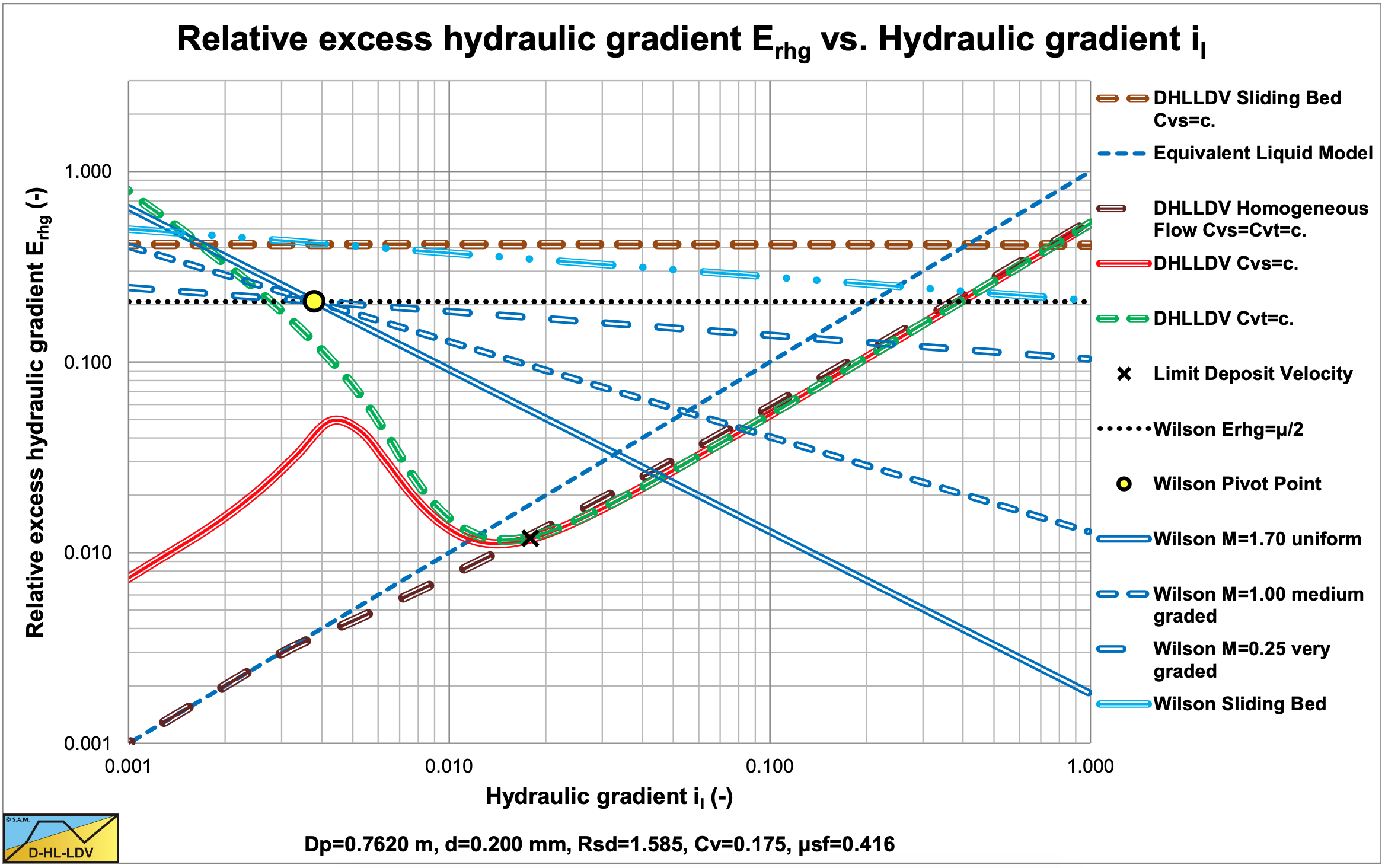
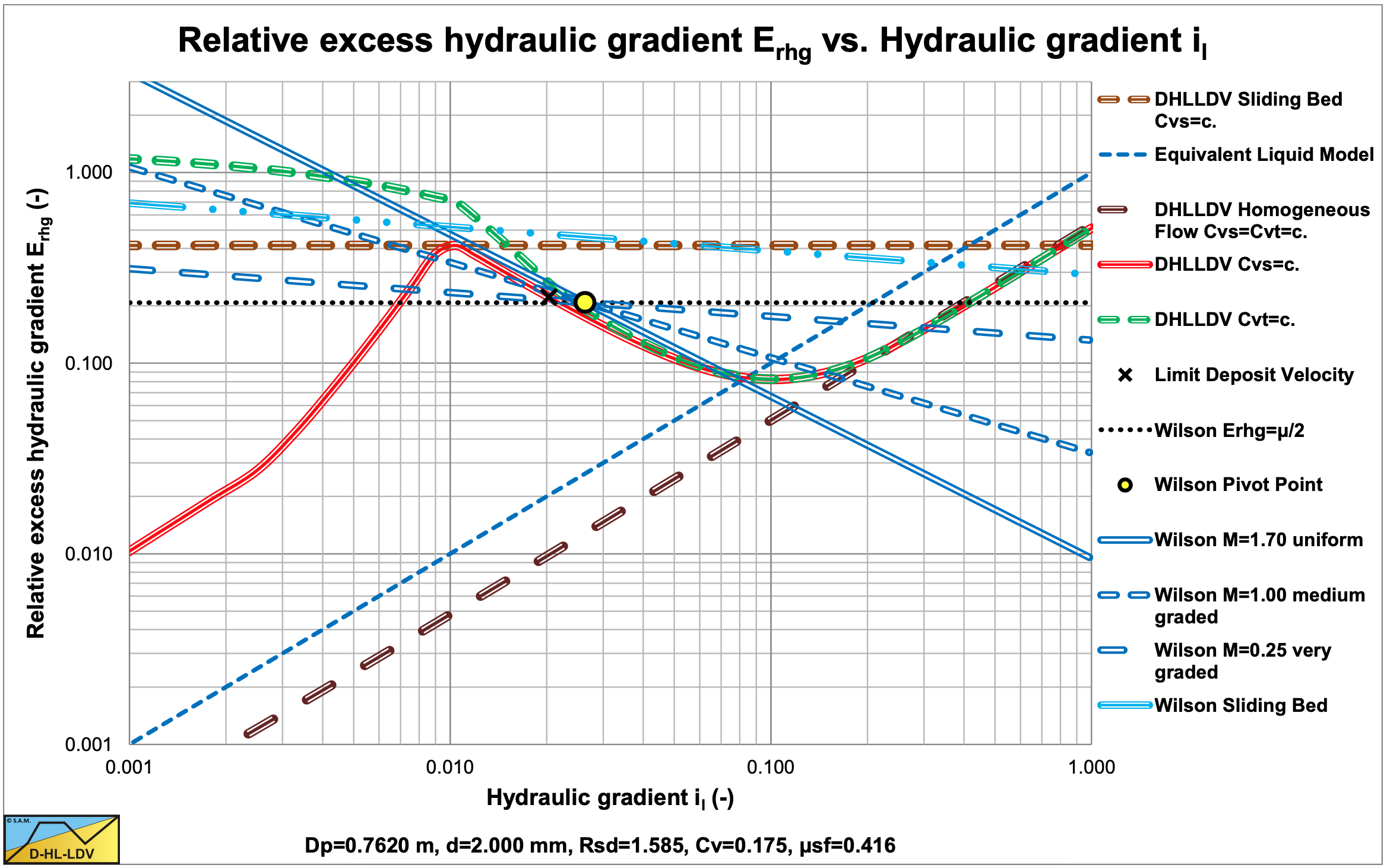
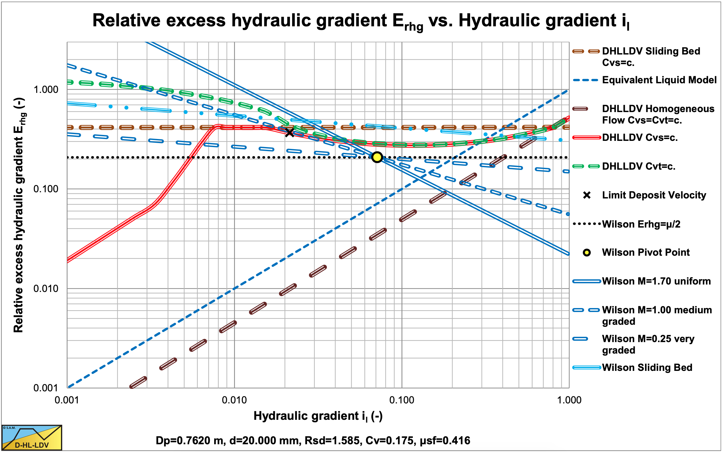
Figure 6.20-21 shows the Wilson et al. (1992) model in E_rhg(i_l) coordinates. The black dotted line is the E_rhg=μ_sf/2 line. The yellow circle the point with v_ls=v₅₀. The heterogeneous Wilson lines have powers of M=1.7, 1.0 & 0.25. So heterogeneous lines always cross the yellow circle, the v₅₀ point, and are rotated around this point depending on the power M. The higher the power M, the steeper the line in this graph.

6.20.2.3 Generic Equation

Based on equation (6.20-53) and equation (6.20-58) and the assumption M=1 for d₈₅/d₅₀=2.72 and assuming the liquid is water of 20 degrees Centigrade and the solids are sand (quarts), an equation is derived to compare Wilson with the other theories:

\[\ \mathrm{i}_{\mathrm{m}}=\mathrm{i}_{\mathrm{l}} \cdot\left(\mathrm{1}+\frac{\mu_{\mathrm{s f}} \cdot \mathrm{g} \cdot \mathrm{R}_{\mathrm{s} \mathrm{d}} \cdot \mathrm{D}_{\mathrm{p}}}{\lambda_{\mathrm{l}}} \cdot\left(\mathrm{v}_{\mathrm{5} 0}\right)^{\mathrm{M}} \cdot\left(\frac{\mathrm{1}}{\mathrm{v}_{\mathrm{ls}}}\right)^{2+\mathrm{M}} \cdot \mathrm{C}_{\mathrm{v}}\right)\]

For the line speed v₅₀:

\[\ \mathrm{v}_{\mathrm{5 0}} \approx \mathrm{3.93} \cdot\left(\mathrm{1 0 0 0} \cdot \mathrm{d}_{\mathrm{5 0}}\right)^{\mathrm{0 . 3 5}}=\mathrm{4 4 . 1} \cdot\left(\mathrm{d}_{\mathrm{5 0}}\right)^{\mathrm{0 . 3 5}}\]

This gives:

\[\ \mathrm{i}_{\mathrm{m}}=\mathrm{i}_{\mathrm{l}} \cdot\left(1+\frac{\mu_{\mathrm{sf}} \cdot \mathrm{g} \cdot \mathrm{R}_{\mathrm{s} \mathrm{d}} \cdot \mathrm{D}_{\mathrm{p}}}{\lambda_{\mathrm{l}}} \cdot\left(44.1 \cdot\left(\mathrm{d}_{50}\right)^{0.35}\right)^{\mathrm{M}} \cdot\left(\frac{\mathrm{1}}{\mathrm{v}_{\mathrm{l s}}}\right)^{2+\mathrm{M}} \cdot \mathrm{C}_{\mathrm{v}}\right)\]

Substituting equation (6.20-61) in equation (6.20-62) gives:

\[\ \mathrm{i}_{\mathrm{m}}=\mathrm{i}_{\mathrm{l}} \cdot\left(\mathrm{1}+\mathrm{4 4 . 1}^{\mathrm{M}} \cdot \frac{\mu_{\mathrm{s f}} \cdot \mathrm{g} \cdot \mathrm{R}_{\mathrm{s d}} \cdot \mathrm{D}_{\mathrm{p}}}{\lambda_{\mathrm{l}}} \cdot\left(\mathrm{d}_{\mathrm{5} 0}\right)^{\mathrm{0 . 3 5} \cdot \mathrm{M}} \cdot\left(\frac{\mathrm{1}}{\mathrm{v}_{\mathrm{l s}}}\right)^{\mathrm{2}+\mathrm{M}} \cdot \mathrm{C}_{\mathrm{v}}\right)\]

With the friction coefficient of μ_sf=0.44, M=1 and some simplifications, this gives:

\[\ \mathrm{i}_{\mathrm{m}}=\mathrm{i}_{\mathrm{l}} \cdot\left(\mathrm{1 + 1 9 . 4} \cdot \frac{\mathrm{g} \cdot \mathrm{R}_{\mathrm{s d}} \cdot \mathrm{D}_{\mathrm{p}}}{\lambda_{\mathrm{l}}} \cdot\left(\mathrm{d}_{50}\right)^{0.35} \cdot\left(\frac{\mathrm{1}}{\mathrm{v}_{\mathrm{l s}}}\right)^{3} \cdot \mathrm{C}_{\mathrm{v}}\right)\]

Giving each term the dimension of velocity gives:

\[\ \mathrm{i}_{\mathrm{m}}=\mathrm{i}_{\mathrm{l}} \cdot\left(\mathrm{1 + 27.64} \cdot \frac{\mathrm{g} \cdot \mathrm{R}_{\mathrm{s d}} \cdot \mathrm{D}_{\mathrm{p}}}{\lambda_{\mathrm{l}}} \cdot\left(\mathrm{g} \cdot \mathrm{d}_{\mathrm{5} 0}\right)^{0.35} \cdot\left(v_{\mathrm{l}} \cdot \mathrm{g}\right)^{0.1} \cdot\left(\frac{\mathrm{1}}{\mathrm{v}_{\mathrm{l s}}}\right)^{\mathrm{3}} \cdot \mathrm{C}_{\mathrm{v}}\right)\]

Or:

\[\ \mathrm{i}_{\mathrm{m}}=\mathrm{i}_{\mathrm{l}}+\mathrm{1 3 . 8 2} \cdot\left(\mathrm{g} \cdot \mathrm{d}_{\mathrm{5 0}}\right)^{\mathrm{0 . 3 5}} \cdot\left(v_{\mathrm{l}} \cdot \mathrm{g}\right)^{\mathrm{0 . 1}} \cdot \frac{\mathrm{1}}{\mathrm{v}_{\mathrm{l} \mathrm{s}}} \cdot \mathrm{R}_{\mathrm{s d}} \cdot \mathrm{C}_{\mathrm{v}}\]

The result is an equation where the excess pressure due to the solids is proportional to the pipe diameter D_p and almost proportional to the cube root of the d₅₀ of the sand. There is no direct relation with the terminal settling velocity v_t or the particle drag coefficient C_D.

6.20.2.4 Analysis of the v₅₀ Equations

The analysis in this chapter is based on the personal interpretation of the author of this book.

Figure 6.20-23 shows data of Durand & Condolios (1952) in the relative excess hydraulic gradient versus the line speed graph. The advantage of this graph is that it show the solids effect in a double logarithmic graph, where curved line become straight lines. The graph also contains the horizontal sliding bed curve (dark brown solid line), the 50% sliding bed curve (black dots), the ELM curve (dashed dark blue line) and the minimum v₅₀ curve (light blue solid line). The intersection line speed of the data series (extrapolated) with the 50% sliding bed curve, the v₅₀, increases with increasing particle diameter. The question is how does it increase?

Based on the assumption that Wilson et al. (1992) developed a model for operation conditions, meaning for operational line speeds. Usually this means line speeds above the Limit Deposit Velocity, or slightly below. In the case considered, see Figure 6.20-23, this gives line speeds of about 2.5 m/s up to 5.5 m/s. Now 3 cases can be considered:

1. Fine particles, d<0.0002 mm.
2. Medium particles, 0.0002<d<1 mm.
3. Coarse particles, d>1 mm.

Fine particles are assumed to be transport according to the homogeneous flow regime under operational conditions. So there is a minimum v₅₀ for particles with a diameter smaller than d=0.0002 mm. The resulting minimum curve is shown in Figure 6.20-23 (the solid light blue curve). This curve is close to the data of the d=0.0002 mm particles. Since Wilson et al. (1992) used different data to calibrate their model, the match is not exactly. This minimum v₅₀ can be determined by:

\[\ \mathrm{v}_{50, \min }=2.7 \cdot\left(\mathrm{R}_{\mathrm{sd}} \cdot \mathrm{g} \cdot v_{\mathrm{l}}\right)^{1 / 3} \cdot \sqrt{\frac{\mathrm{8}}{\lambda_{\mathrm{l}}}} \quad\text{ or }\quad \mathrm{v}_{50, \min }=\frac{1}{\mu_{\mathrm{sf}}} \cdot\left(\mathrm{R}_{\mathrm{sd}} \cdot \mathrm{g} \cdot v_{\mathrm{l}}\right)^{1 / 3} \cdot \sqrt{\frac{\mathrm{8}}{\lambda_{\mathrm{l}}}}\]

Figure 6.20-23: The data of Durand & Condolios (1952).

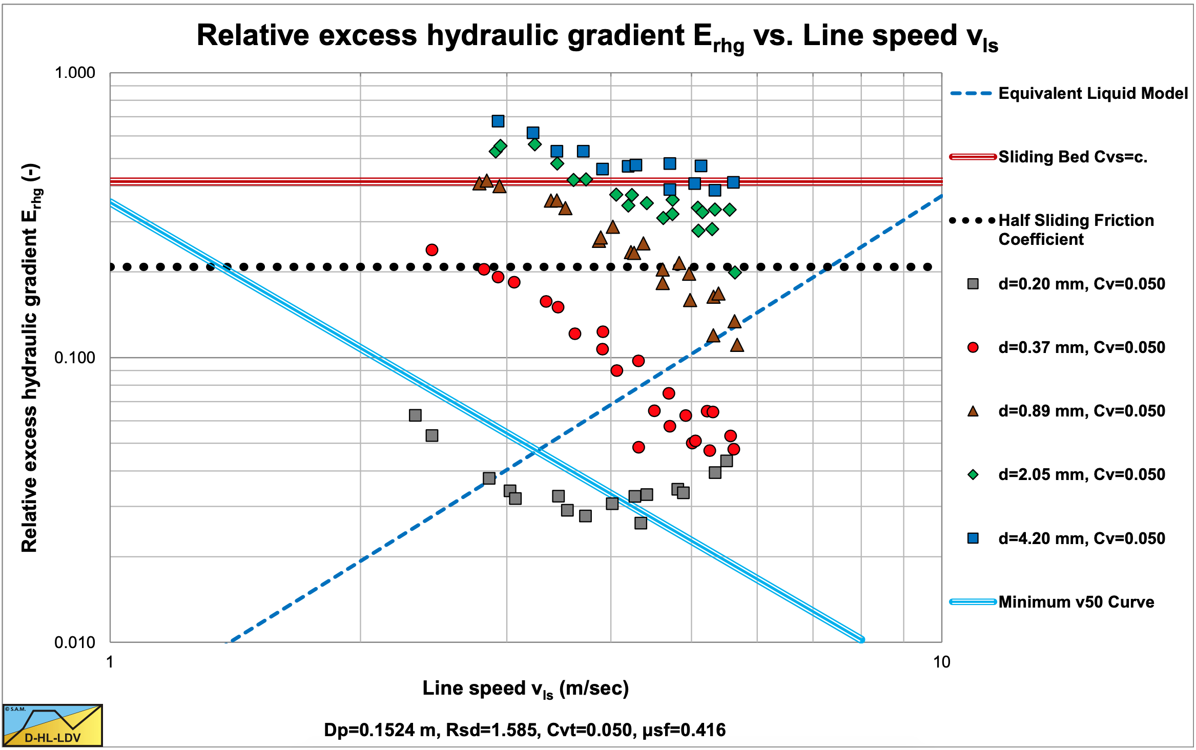
For medium sized particles, the v₅₀ is increasing. Figure 6.20-23 shows this increase for particles with d=0.37 mm and d=0.89 mm. Wilson et al. (1992) assumed this increase is proportional to the terminal settling velocity v_t. This gives:

\[\ \mathrm{v}_{50}=\left(0.9 \cdot \mathrm{v}_{\mathrm{t}}+2.7 \cdot\left(\mathrm{R}_{\mathrm{sd}} \cdot \mathrm{g} \cdot v_{\mathrm{l}}\right)^{1 / 3}\right) \cdot \sqrt{\frac{8}{\lambda_{\mathrm{l}}}}\quad\text{ or }\quad\mathrm{v}_{50}=\left(0.9 \cdot \mathrm{v}_{\mathrm{t}}+\frac{1}{\mu_{\mathrm{sf}}} \cdot\left(\mathrm{R}_{\mathrm{sd}} \cdot \mathrm{g} \cdot v_{\mathrm{l}}\right)^{1 / 3}\right) \cdot \sqrt{\frac{8}{\lambda_{\mathrm{l}}}}\]

For coarse particles, the steepness of the decrease of the E_rhg parameter with increasing line speed v_ls is less than for medium particles. In fact it looks like the larger the particle, the less steep the decrease, where very coarse particles could result in an almost horizontal curve. This also means that the intersection line speed of the extrapolated data points with the 50% sliding bed curve is more far away. A horizontal curve has an intersection v₅₀ at infinity. Wilson et al. (1992) took this behavior into account by adding a term with the particle diameter to pipe diameter ratio, according to:

\[\ \mathrm{v}_{50}=\left(0.9 \cdot \mathrm{v}_{\mathrm{t}}+2.7 \cdot\left(\mathrm{R}_{\mathrm{sd}} \cdot \mathrm{g} \cdot v_{\mathrm{l}}\right)^{1 / 3}\right) \cdot \sqrt{\frac{8}{\lambda_{\mathrm{l}}}} \cdot \cosh \left(\frac{\mathrm{6 0} \cdot \mathrm{d}_{50}}{\mathrm{D}_{\mathrm{p}}}\right)\]

The Darcy Weisbach friction coefficient λ_l indirectly gives the influence of the pipe diameter. The cosh term gives the influence of the particle diameter to pipe diameter ratio. Figure 6.20-24 shows the resulting v₅₀ curve for a D_p=0.1524 m pipe (6 inch) (the thick black solid line).

\[\ \mathrm{E}_{\mathrm{r h g}}=\mathrm{R}=\frac{\mathrm{i}_{\mathrm{m}}-\mathrm{i}_{\mathrm{l}}}{\mathrm{R}_{\mathrm{s d}} \cdot \mathrm{C}_{\mathrm{v}}}=\frac{\Delta \mathrm{p}_{\mathrm{m}}-\Delta \mathrm{p}_{\mathrm{l}}}{\rho_{\mathrm{l}} \cdot \mathrm{g} \cdot \Delta \mathrm{L} \cdot \mathrm{R}_{\mathrm{s d}} \cdot \mathrm{C}_{\mathrm{v}}}=\frac{\mu_{\mathrm{s f}}}{\mathrm{2}} \cdot\left(\frac{\mathrm{v}_{\mathrm{5 0}}}{\mathrm{v}_{\mathrm{l s}}}\right)^{\mathrm{M}}\]

For uniform sands Wilson et al. (1992) found a power M=1.7 in the above equation, which works well for medium sands, however for the coarser sands the effect of the cosh term in the v₅₀ should be accompanied by a decrease of this power as follows from the data in Figure 6.20-23. Durand & Condolios (1952) found that for coarse particles the hydraulic gradient and thus the E_rhg parameter does not really increase, based on the particle Froude number. The definition of coarse is related to the pipe diameter by Wilson et al. (1992) being d=0.015·D_p or d=D_p/60. This gives for the v₅₀:

\[\ \mathrm{v}_{50^{*}}=\left(0.9 \cdot \mathrm{v}_{\mathrm{t}^{*}}+2.7 \cdot\left(\mathrm{R}_{\mathrm{sd}} \cdot \mathrm{g} \cdot v_{\mathrm{l}}\right)^{1 / 3}\right) \cdot \sqrt{\frac{8}{\lambda_{\mathrm{l}}}} \cdot \cosh (1)\]

The line speed where the heterogeneous curve intersects with the sliding bed curve is about:

\[\ \mathrm{v}_{\mathrm{l s}^{*}}=\frac{\mathrm{2}}{\mathrm{3}} \cdot \mathrm{v}_{\mathrm{5 0}^{*}}\]

Now assume this line speed is a constant, given a certain pipe diameter, the power M for particles of d>0.015^.D_p is:

\[\ \mathrm{M}=\frac{\ln (2)}{\ln \left(\frac{3}{2} \cdot \frac{\mathrm{v}_{50}}{\mathrm{v}_{50^{*}}}\right)}\]

In these equations the * is used for the particle diameter d>0.015·D_p. This approach leads to a continuous behavior of the heterogeneous flow regime.

Figure 6.20-25: The v₅₀ curves for a D_p=0.4 m pipe.

Wilson et al. (1992) simplified the v₅₀ equation to:

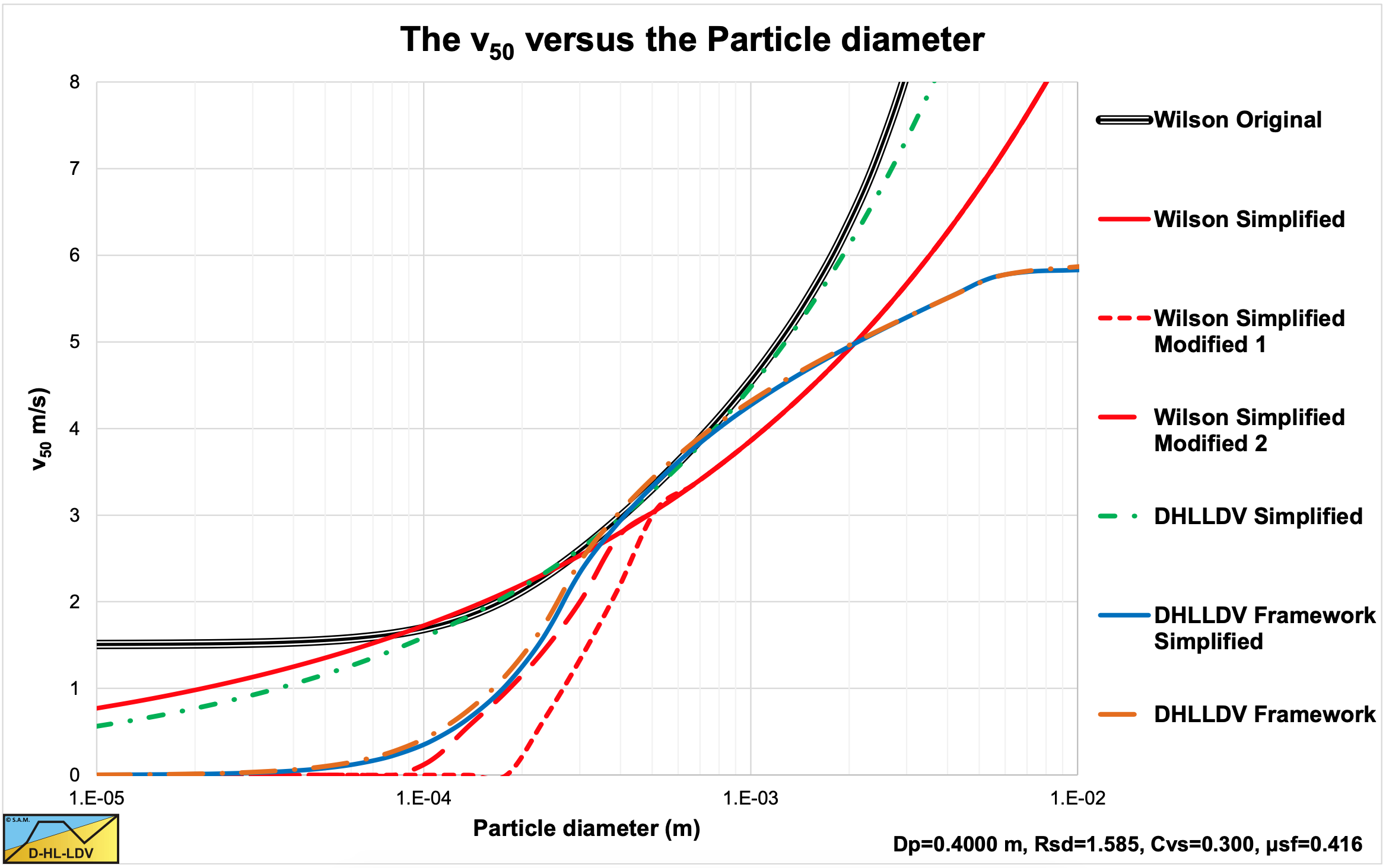
\[\ \mathrm{v}_{\mathrm{5 0}} \approx \mathrm{3 . 9 3} \cdot\left(\frac{\mathrm{d}_{\mathrm{5 0}}}{\mathrm{0 . 0 0 1}}\right)^{\mathrm{0 . 3 5}} \cdot\left(\frac{\mathrm{R}_{\mathrm{s d}}}{\mathrm{1.65}}\right)^{\mathrm{0 . 4 5}} \cdot\left(\frac{v_{\mathrm{l}, \mathrm{a c t u a l}}}{v_{\mathrm{w}, \mathrm{2 0}}}\right)^{-\mathrm{0 . 2 5}}\]

Giving a v₅₀ of 3.93 m/s for a 1 mm sand particle in 20o water. This simplified equation is also shown in Figure 6.20-24 (the solid red line). This equation does not contain the influence of the pipe diameter and only approaches the original equation for medium sands. Later the simplified equation has been adjusted for particles with diameters from 0.2 mm to 0.5 mm with a factor:

\[\ \mathrm{f=\frac{d_{h}-0.0002}{0.0005-0.0002}}\]

This is also shown in Figure 6.20-24 as the Wilson simplified modified curve (dashed red line). Where the original equation seems to overestimate the solids effect of fine particles, this modification seems to underestimate the solids effect.

Figure 6.20-24, Figure 6.20-25 and Figure 6.20-26 show the original v₅₀ method, the simplified and the simplified modified equations. The effect of not having the pipe diameter influence in the simplified and the simplified modified equations results in a deviation of these equations with the original method for large diameter pipes.

Figure 6.20-26: The v₅₀ curves for a D_p=1.2 m pipe.

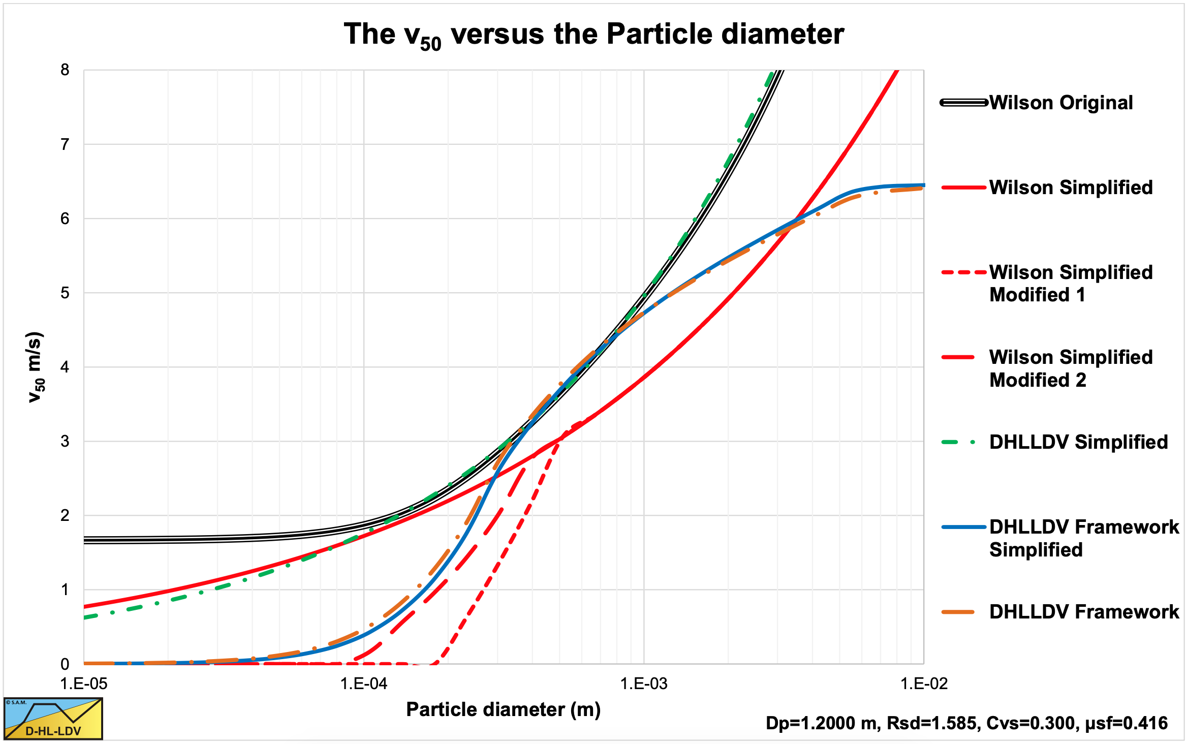
A better simplification of the v₅₀ is achieved with the following equation (DHLLDV simplified, the solid green line):

\[\ \mathrm{v}_{\mathrm{5 0}} \approx \mathrm{3} \cdot\left(\frac{\mathrm{d}_{\mathrm{5 0}}}{\mathrm{0 .0 0 0 5}}\right)^{\mathrm{0 .4 5}} \cdot\left(\frac{\mathrm{R}_{\mathrm{s d}}}{\mathrm{1 .6 5}}\right)^{\mathrm{0 .4 5}} \cdot\left(\frac{\mathrm{v}_{\mathrm{l}, \mathrm{a c t u a l}}}{v_{\mathrm{w}, \mathrm{2 0}}}\right)^{-\mathrm{0 .2 5}} \cdot\left(\frac{\mathrm{D}_{\mathrm{p}}}{\mathrm{0 .1 5 2 4}}\right)^{\mathrm{0 . 0 9 2}}\]

Figure 6.20-24, Figure 6.20-25 and Figure 6.20-26 show this equation as well. For a D_p=0.1524 m (6 inch) pipe, this equation gives an almost identical v₅₀ compared to the original method for particle diameters in the range of 0.1 to 0.8 mm. For the D_p=0.4 m pipe this range is larger, from 0.1 to 2 mm. For the D_p=1.2 m the range is even larger than for the D_p=0.4 m pipe, the approximation is valid for particles with a diameter from 0.1 mm and above. Still the overestimation of the v₅₀ for small particles remains, as a result of the original assumption of Wilson that there is a minimum v₅₀. Figure 6.20-35 shows that also particles with a diameter smaller than 0.1 mm show heterogeneous behavior with a v₅₀ much smaller than this minimum v₅₀. The correction with equation (6.20-75) seems too drastic and not at the right location. The following correction factor in the range of particle diameters from 0.1 to 0.3 mm seems more appropriate and approaches the DHLLDV curves closely.

\[\ \mathrm{f}=\frac{\mathrm{d}_{\mathrm{h}}-\mathrm{0 . 0 0 0 1}}{\mathrm{0 .0 0 0 4 - 0 . 0 0 0 1}}\]

A better approach of the v₅₀ however is the following equation, based on the DHLLDV Framework:

\[\ \mathrm{v}_{50} \approx 3.4 \cdot\left(\frac{\mathrm{v}_{\mathrm{t}}}{\sqrt{\mathrm{g} \cdot \mathrm{d}}}\right)^{1.96} \cdot\left(\frac{\mathrm{D}_{\mathrm{p}}}{\mathrm{0 .1 5 2 4}}\right)^{0.092} \cdot\left(\frac{\mathrm{R}_{\mathrm{s d}}}{\mathrm{1 .6 5}}\right)^{-\mathrm{0 . 0 9 2}} \cdot\left(\frac{v_{\mathrm{l}, \mathrm{a c t u a l}}}{v_{\mathrm{w}, \mathrm{2 0}}}\right)^{0.27}\]

Figure 6.20-24, Figure 6.20-25 and Figure 6.20-26 show the results of this equation and also the results of the much more complicated DHLLDV Framework. In the range of particle diameters of 0.3 to 1 mm, this equation matches the original Wilson method very closely. Above 1 mm the original Wilson method goes to infinity (because of the decreasing power M), while the DHLLDV simplified equation goes to a constant value (assuming the power M does not change) matching the findings of Durand & Condolios (1952). For particles with a diameter smaller than 0.3 mm this equation matches many experimental data and solves the problem of overestimation of the original Wilson method in a more structural way.

6.20.2.5 Conclusions & Discussion

The basic form of the equation for heterogeneous transport, equation (6.20-51), is of the type; hydraulic gradient mixture equals hydraulic gradient carrier liquid + solids effect. This implies that the hydraulic gradient of the carrier liquid and the solids effect are independent like in the Fuhrboter (1961) model. This in contrary with the Durand & Condolios (1952), Newitt et al. (1955) and the Jufin & Lopatin (1966) models. These are of the type; hydraulic gradient mixture equals hydraulic gradient carrier liquid times 1 + solids effect. Equations (6.20-65) and (6.20-66) show the Wilson equation for both types, with correct dimensions.

Basically the model shows straight lines in the E_rhg(i_l) graph with the v₅₀, 0.22 point as a pivot point. Depending on the value of the power M, the straight line pivots around this point. Figure 6.20-21 shows these straight line for powers of 0.25, 1.0 and 1.7. The power of 1.7 for uniform sands matches very well with the DHLLDV Framework for uniform sands.

The model gives good results if the physics on which it is based occur, medium sized particles. For very fine particles in a large pipe there will never be a sliding bed. The stationary bed will vaporize (erode) with increasing line speed, probably without sheet flow, see Figure 6.20-20. The 50% stratification criterion is not valid here because the sliding friction is not 100% mobilized resulting in a much lower friction. Very large particles will, almost always, be more than 50% stratified, resulting in a sliding bed or sliding flow, so the model is also invalid in this case, see Figure 6.20-22.

The DHLLDV simplified equation gives a much better approximation of the v₅₀ parameter and solved a number of shortcomings.

Wilson et al. (2006) suggests the following equation for full stratified flow, based on μ_sf=0.4 (or 0.44):

\[\ \begin{array}{rl}\mathrm{i}_{\mathrm{m}}=\mathrm{i}_{\mathrm{l}}+\mathrm{C}_{\mathrm{v} \mathrm{t}} \cdot \mathrm{R}_{\mathrm{s} \mathrm{d}} \cdot \mathrm{2} \cdot \mathrm{\mu}_{\mathrm{s f}} \cdot\left(\frac{\mathrm{4} \cdot \mathrm{v}_{\mathrm{s m}}}{\mathrm{3} \cdot \mathrm{v}_{\mathrm{l} \mathrm{s}}}\right)^{\mathrm{0 . 2 5}} & \mathrm{o r} \quad \mathrm{i}_{\mathrm{m}}=\mathrm{i}_{\mathrm{l}}+\mathrm{C}_{\mathrm{v t}} \cdot \mathrm{R}_{\mathrm{s d}} \cdot \mathrm{2} \cdot \mu_{\mathrm{s f}} \cdot\left(\frac{\mathrm{v}_{\mathrm{s m}}}{\mathrm{v}_{\mathrm{l s}}}\right)^{\mathrm{0 . 2 5}} \\ \text { Based on } \mu_{\mathrm{s f}}=\mathrm{0 . 4 0}\quad\quad\quad\quad & \quad\quad\quad\quad\text{ Based on } \mu_{\mathrm{s f}}=\mathrm{0 . 4 4}\end{array}\]

As is shown in Figure 6.20-22 there will be a discontinuity jumping from the heterogeneous model to the full stratified model, even if the same power of 0.25 is applied. In fact if more than 50% of the solids is stratified, the v₅₀ point at E_rhg=0.22 in the 3 graphs will never be reached.

In a number of papers the fully stratified flow term is reduced to 50% or even 25%, so it is not really clear what to use. Assuming a full sliding bed at the Limit of Stationary Deposity Velocity, the equation should be for the constant spatial volumetric case and based on the weight approach:

\[\ \mathrm{i}_{\mathrm{m}}=\mathrm{i}_{\mathrm{l}}+\mathrm{C}_{\mathrm{v s}} \cdot \mathrm{R}_{\mathrm{s d}} \cdot \mu_{\mathrm{s f}} \cdot\left(\frac{\mathrm{v}_{\mathrm{s m}}}{\mathrm{v}_{\mathrm{l s}}}\right)^{\mathrm{0 . 2 5}}\]

For the constant delivered volumetric case this gives:

\[\ \mathrm{i}_{\mathrm{m}}=\mathrm{i}_{\mathrm{l}}+\frac{\mathrm{C}_{\mathrm{v s}}\left(\mathrm{v}_{\mathrm{s m}}\right)}{\mathrm{C}_{\mathrm{vt}}} \cdot \mathrm{C}_{\mathrm{v t}} \cdot \mathrm{R}_{\mathrm{s d}} \cdot \mu_{\mathrm{s f}} \cdot\left(\frac{\mathrm{v}_{\mathrm{s m}}}{\mathrm{v}_{\mathrm{l} \mathrm{s}}}\right)^{\mathrm{0 . 2 5}}\]

Where the spatial concentration at the LSDV depends on the line speed and other parameters, but is always larger than 1.

6.20.3 The 4 Component Model of Wilson & Sellgren (2001)

6.20.3.1 Introduction

Broad particle grading mean that several of the normally considered slurry flow regimes are included. A pipeline slurry friction loss model consisting of three regimes was initially proposed by K.C. Wilson in (2001), then extended to a four components consisting of fluid, pseudo-homogeneous, heterogeneous and fully stratified components, Wilson et al. (2006). It was successively developed and validated for a variety of experimental data covering volumetric solids concentrations of up to nearly 40% and particle sizes of up to 65mm, Sellgren and Wilson (2007).

Four components are distinguished:

1. Homogeneous flow (uses the index f), the fraction d<0.04 mm.
2. Pseudo homogeneous flow (uses the index ph), the fraction 0.04 mm<d<0.2·\(\ v_r \) mm.
3. Heterogeneous flow (uses the index h), the fraction 0.2·ν_r mm<d<0.015·D_p.
4. Stratified flow (uses the index s), d>0.015·D_p.

The relative kinematic viscosity \(\ v_r \) is the ratio of the kinematic viscosity of the carrier fluid to that of water at 20°C.

The sum of the 4 fractions always has to be equal to unity.

\[\ \mathrm{X}_{\mathrm{f}}+\mathrm{X}_{\mathrm{p h}}+\mathrm{X}_{\mathrm{h}}+\mathrm{X}_{\mathrm{s}}=\mathrm{1}\]

The total delivered volumetric concentration is the sum of the concentrations of the 4 fractions.

\[\ \mathrm{C}_{\mathrm{v t}}=\mathrm{C}_{\mathrm{v t}, \mathrm{f}}+\mathrm{C}_{\mathrm{v} \mathrm{t}, \mathrm{p h}}+\mathrm{C}_{\mathrm{v} \mathrm{t}, \mathrm{h}}+\mathrm{C}_{\mathrm{v} \mathrm{t}, \mathrm{s}}=\mathrm{X}_{\mathrm{f}} \cdot \mathrm{C}_{\mathrm{v t}}+\mathrm{X}_{\mathrm{p h}} \cdot \mathrm{C}_{\mathrm{v t}}+\mathrm{X}_{\mathrm{h}} \cdot \mathrm{C}_{\mathrm{v t}}+\mathrm{X}_{\mathrm{s}} \cdot \mathrm{C}_{\mathrm{vt}}\]

The total hydraulic gradient of the mixture is the sum of the hydraulic (excess) gradients of the 4 fractions.

\[\ \mathrm{i}_{\mathrm{m}}=\mathrm{i}_{\mathrm{f}}+\Delta \mathrm{i}_{\mathrm{p h}}+\Delta \mathrm{i}_{\mathrm{h}}+\Delta \mathrm{i}_{\mathrm{s}} \quad\text{ in }\quad(\mathrm{m} \text { carrier liquid/m pipe })\]

6.20.3.2 The Homogeneous or Equivalent Fluid Fraction

In the homogeneous phase, the spatial and transport volumetric concentrations are assumed to be equal.

\[\ \mathrm{C}_{\mathrm{v s}, \mathrm{f}}=\mathrm{C}_{\mathrm{v t}, \mathrm{f}}\]

Thomas (1965) derived an equation to determine the effective viscosity μ_f as a function of the concentration C_vs,f of the particles in the mixture:

\[\ \mu_{\mathrm{f}}=\mu_{\mathrm{l}} \cdot\left(1+2.5 \cdot \mathrm{C}_{\mathrm{vs}, \mathrm{f}}+10.05 \cdot \mathrm{C}_{\mathrm{vs}, \mathrm{f}}^{2}+0.00273 \cdot \mathrm{e}^{16.6 \cdot \mathrm{C}_{\mathrm{vs}, \mathrm{f}}}\right) \quad\text{ with: }\quad \mu_{\mathrm{r}}=\mu_{\mathrm{f}} / \mu_{\mathrm{l}}\]

The fluid density ρ_f equals the carrier liquid density ρ_l plus the additional density of the homogeneous fraction of the PSD, according to Wilson et al. (2006) the fraction smaller than 0.04 mm.

\[\ \rho_{\mathrm{f}}=\rho_{\mathrm{l}} \cdot\left(1+\mathrm{R}_{\mathrm{s d}} \cdot \mathrm{C}_{\mathrm{v s}, \mathrm{f}}\right) \quad\text{ and }\quad v_{\mathrm{f}}=\frac{\mu_{\mathrm{f}}}{\rho_{\mathrm{f}}}\]

This results in modified fluid properties compared with the carrier liquid, which will be used for all the flow regimes. The hydraulic gradient of the homogeneous flow regime i_f is now:

\[\ \mathrm{i}_{\mathrm{l}}=\frac{\lambda_{\mathrm{f}} \cdot \mathrm{v}_{\mathrm{l s}}^{2}}{2 \cdot \mathrm{g} \cdot \mathrm{D}_{\mathrm{p}}} \Rightarrow \mathrm{i}_{\mathrm{f}}=\frac{\Delta \mathrm{p}_{\mathrm{f}}}{\rho_{\mathrm{l}} \cdot \mathrm{g} \cdot \Delta \mathrm{L}}=\frac{\rho_{\mathrm{f}}}{\rho_{\mathrm{l}}} \cdot \frac{\lambda_{\mathrm{f}} \cdot \mathrm{v}_{\mathrm{l} \mathrm{s}}^{2}}{\mathrm{2} \cdot \mathrm{g} \cdot \mathrm{D}_{\mathrm{p}}}=\frac{\rho_{\mathrm{f}}}{\rho_{\mathrm{l}}} \cdot \mathrm{i}_{\mathrm{l}} \quad\text{ with: }\quad \Delta \mathrm{p}_{\mathrm{f}}=\lambda_{\mathrm{f}} \cdot \frac{\Delta \mathrm{L}}{\mathrm{D}_{\mathrm{p}}} \cdot \frac{1}{2} \cdot \rho_{\mathrm{f}} \cdot \mathrm{v}_{\mathrm{ls}}^{\mathrm{2}}\]

The Darcy Weisbach friction factor λ_f is determined based on these fluid properties. The Darcy Weisbach friction factor will not differ much from the Darcy Weisbach friction factor resulting from the carrier liquid properties.

6.20.3.3 The Pseudo Homogeneous Fraction

In the pseudo homogeneous phase, the spatial and transport volumetric concentrations are also assumed to be equal.

\[\ \mathrm{C_{v s, p h}=C_{v t, p h}}\]

The hydraulic gradient Δi_ph is determined with the ELM model without adjusting the effective viscosity according to:

\[\ \Delta \mathrm{i}_{\mathrm{ph}}=\mathrm{C}_{\mathrm{vs}, \mathrm{ph}} \cdot\left(\frac{\rho_{\mathrm{s}}-\rho_{\mathrm{f}}}{\rho_{\mathrm{f}}}\right) \cdot \mathrm{i}_{\mathrm{f}}=\mathrm{C}_{\mathrm{vs}, \mathrm{ph}} \cdot\left(\frac{\rho_{\mathrm{s}}-\rho_{\mathrm{f}}}{\rho_{\mathrm{f}}}\right) \cdot \frac{\rho_{\mathrm{f}}}{\rho_{\mathrm{l}}} \cdot \mathrm{i}_{\mathrm{l}}=\mathrm{C}_{\mathrm{vs}, \mathrm{ph}} \cdot\left(\frac{\rho_{\mathrm{s}}-\rho_{\mathrm{f}}}{\rho_{\mathrm{l}}}\right) \cdot \mathrm{i}_{\mathrm{l}}\]

The resulting density ρ_fp for the next flow regime is:

\[\ \rho_{\mathrm{fp}}=\rho_{\mathrm{l}} \cdot\left(1+\mathrm{R}_{\mathrm{sd}} \cdot \mathrm{C}_{\mathrm{v s}, \mathrm{f}}+\mathrm{R}_{\mathrm{sd}} \cdot \mathrm{C}_{\mathrm{v s}, \mathrm{p h}}\right)\]

The fluid viscosity is not adjusted for the density or concentration in this fraction.

6.20.3.4 The Heterogeneous Fraction

The original Wilson et al. (2006) heterogeneous model is based on a velocity v₅₀, where 50% of the solids are stratified and the other 50% in suspension. The simplified equation to determine this v₅₀ is:

\[\ \mathrm{v}_{\mathrm{5 0}} \approx \mathrm{3 .9 3} \cdot\left(\mathrm{1 0 0 0} \cdot \mathrm{d}_{\mathrm{5 0}}\right)^{\mathrm{0 . 3 5}} \cdot\left(\frac{\mathrm{R}_{\mathrm{s d}}}{\mathrm{1 .6 5}}\right)^{\mathrm{0 . 4 5}} \cdot\left(\frac{v_{\mathrm{f}}}{v_{\mathrm{l}, \mathrm{2} 0}}\right)^{-\mathrm{0 . 2 5}}\]

The original equation to determine the excess hydraulic gradient is:

\[\ \Delta \mathrm{i}_{\mathrm{h}}=\mathrm{C}_{\mathrm{v} \mathrm{t}} \cdot \mathrm{R}_{\mathrm{s} \mathrm{d}} \cdot \frac{\boldsymbol{\mu}_{\mathrm{s} \mathrm{f}}}{\mathrm{2}} \cdot\left(\frac{\mathrm{v}_{\mathrm{5 0}}}{\mathrm{v}_{\mathrm{l s}}}\right)^{\mathrm{M}}\]

The equation for v₅₀ now has to be adjusted for an average particle diameter of the heterogeneous fraction d_h and for the relative submerged density according to:

\[\ \begin{array}{left} \mathrm{v}_{\mathrm{5 0}} \approx \mathrm{3.93} \cdot\left(\mathrm{1 0 0 0} \cdot \mathrm{d}_{\mathrm{h}}\right)^{\mathrm{0 . 3 5}} \cdot\left(\frac{\rho_{\mathrm{s}}-\rho_{\mathrm{f p}}}{\rho_{\mathrm{l}}} \cdot \frac{\mathrm{1}}{\mathrm{1 . 6 5}}\right)^{\mathrm{0 .4 5}} \cdot v_{\mathrm{r}}^{-\mathrm{0 . 2 5}}\\
\mathrm{d}_{\mathrm{h}}=\frac{\left(\mathrm{0 . 0 0 0 2} \cdot v_{\mathrm{r}}+\mathrm{M i n}\left(\mathrm{0 . 0 1 5} \cdot \mathrm{D}_{\mathrm{p}}, \mathrm{d}_{\mathrm{m a x}}\right)\right)}{\mathrm{2}}\end{array}\]

The excess hydraulic gradient Δi_h can now be determined according to, where M is taken as unity:

\[\ \begin{array}\Delta \mathrm{i}_{\mathrm{h}}=\frac{\rho_{\mathrm{f p}}}{\rho_{\mathrm{l}}} \cdot \mathrm{C}_{\mathrm{v} \mathrm{t}, \mathrm{h}} \cdot\left(\frac{\rho_{\mathrm{s}}-\rho_{\mathrm{f p}}}{\rho_{\mathrm{f p}}}\right) \cdot \frac{\mu_{\mathrm{s} \mathrm{f}}}{2} \cdot\left(\frac{\mathrm{v}_{\mathrm{5} 0}}{\mathrm{v}_{\mathrm{ls}}}\right)^{\mathrm{M}}\\
\mathrm{O} \mathrm{r}\\
\Delta \mathrm{i}_{\mathrm{h}}=\frac{\rho_{\mathrm{f p}}}{\rho_{\mathrm{l}}} \cdot \mathrm{C}_{\mathrm{v} \mathrm{t}, \mathrm{h}} \cdot\left(\frac{\rho_{\mathrm{s}}-\rho_{\mathrm{f p}}}{\rho_{\mathrm{f p}}}\right) \cdot \frac{\mu_{\mathrm{s f}}}{2} \cdot\left(\frac{\mathrm{v}_{\mathrm{5} 0}}{\mathrm{v}_{\mathrm{l s}}}\right)^{\mathrm{M}} \cdot \frac{\mathrm{d}_{\mathrm{h}}-\mathrm{0 . 0 0 0 2}}{\mathrm{0 . 0 0 0 5 - 0 . 0 0 0 2}} \quad\text{ for }\quad \mathrm{0 . 0 0 0 2 < d}_{\mathrm{h}}<\mathrm{0 . 0 0 0 5}\end{array}\]

The resulting density for the next flow regime is:

\[\ \rho_{\mathrm{fph}}=\rho_{\mathrm{l}} \cdot\left(1+\mathrm{R}_{\mathrm{sd}} \cdot \mathrm{C}_{\mathrm{v s}, \mathrm{f}}+\mathrm{R}_{\mathrm{s d}} \cdot \mathrm{C}_{\mathrm{v s}, \mathrm{p h}}+\mathrm{R}_{\mathrm{s d}} \cdot \mathrm{C}_{\mathrm{v s}, \mathrm{h}}\right)\]

6.20.3.5 The Fully Stratified Fraction

In the original model of Wilson et al. (2006) the maximum limit of stationary deposit velocity v_sm can be estimated by:

\[\ \mathrm{v}_{\mathrm{sm}}=\frac{\mathrm{8.8} \cdot\left(\frac{\mu_{\mathrm{sf}} \cdot \mathrm{R}_{\mathrm{sd}}}{\mathrm{0.66}}\right)^{0.55} \cdot \mathrm{D}_{\mathrm{p}}^{0.7} \cdot \mathrm{d}^{\mathrm{1 . 7 5}}}{\mathrm{d}^{2}+\mathrm{0.1 1} \cdot \mathrm{D}_{\mathrm{p}}^{0.7}}\]

The original excess hydraulic gradient for a fully stratified flow can be approximated by (for a friction coefficient of 0.4):

\[\ \Delta \mathrm{i}_{\mathrm{s}}=\mathrm{C}_{\mathrm{v t}} \cdot \mathrm{R}_{\mathrm{s d}} \cdot \mathrm{2} \cdot \mu_{\mathrm{s f}} \cdot\left(\frac{\mathrm{v}_{\mathrm{s m}}}{\mathrm{v}_{\mathrm{l s}}}\right)^{\mathrm{0 . 2 5}}\]

Wilson et al. (2006) suggest to multiply this equation by 0.5, adjust the relative submerged density, not to adjust V_sm and of course use the strtified fraction according to:

\[\ \Delta \mathrm{i}_{\mathrm{s}}=\frac{\rho_{\mathrm{fph}}}{\rho_{\mathrm{l}}} \cdot \mathrm{C}_{\mathrm{v} \mathrm{t}, \mathrm{s}} \cdot\left(\frac{\rho_{\mathrm{s}}-\rho_{\mathrm{f p h}}}{\rho_{\mathrm{f p h}}}\right) \cdot \mu_{\mathrm{s f}} \cdot\left(\frac{\mathrm{v}_{\mathrm{s m}}}{\mathrm{v}_{\mathrm{l s}}}\right)^{0.25}\]

The resulting mixture density is now:

\[\ \rho_{\mathrm{m}}=\rho_{\mathrm{l}} \cdot\left(1+\mathrm{R}_{\mathrm{s d}} \cdot \mathrm{C}_{\mathrm{v s}, \mathrm{f}}+\mathrm{R}_{\mathrm{s d}} \cdot \mathrm{C}_{\mathrm{v s}, \mathrm{p} \mathrm{h}}+\mathrm{R}_{\mathrm{s d}} \cdot \mathrm{C}_{\mathrm{v s}, \mathrm{h}}+\mathrm{R}_{\mathrm{s d}} \cdot \mathrm{C}_{\mathrm{v s , s}}\right)=\rho_{\mathrm{l}} \cdot\left(\mathrm{1}+\mathrm{R}_{\mathrm{s d}} \cdot \mathrm{C}_{\mathrm{v s}}\right)\]

6.20.3.6 The Resulting Equation

The resulting equation of the 4 component model is:

\[\ \begin{aligned} \mathrm{i}_{\mathrm{m}}=& \frac{\rho_{\mathrm{f}}}{\rho_{\mathrm{l}}} \cdot \frac{\lambda_{\mathrm{f}} \cdot \mathrm{v}_{\mathrm{l} \mathrm{s}}^{2}}{\mathrm{2} \cdot \mathrm{g} \cdot \mathrm{D}_{\mathrm{p}}} \cdot\left(\mathrm{1}+\mathrm{C}_{\mathrm{v} \mathrm{t}, \mathrm{p h}} \cdot\left(\frac{\rho_{\mathrm{s}}-\rho_{\mathrm{f}}}{\rho_{\mathrm{f}}}\right)\right)+\frac{\rho_{\mathrm{f p}}}{\rho_{\mathrm{l}}} \cdot \mathrm{C}_{\mathrm{v} \mathrm{t}, \mathrm{h}} \cdot\left(\frac{\rho_{\mathrm{s}}-\rho_{\mathrm{f p}}}{\rho_{\mathrm{f p}}}\right) \cdot \frac{\mu_{\mathrm{f f}}}{\mathrm{2}} \cdot\left(\frac{\mathrm{v}_{\mathrm{5} 0}}{\mathrm{v}_{\mathrm{l s}}}\right)^{\mathrm{M}} +\frac{\rho_{\mathrm{fph}}}{\rho_{\mathrm{l}}} \cdot \mathrm{C}_{\mathrm{v} \mathrm{t}, \mathrm{s}} \cdot\left(\frac{\rho_{\mathrm{s}}-\rho_{\mathrm{f p h}}}{\rho_{\mathrm{f p h}}}\right) \cdot \mu_{\mathrm{sf}} \cdot\left(\frac{\mathrm{v}_{\mathrm{s m}}}{\mathrm{v}_{\mathrm{l s}}}\right)^{0.25} \end{aligned}\]

The way the different mixture densities are determined is incorrect. For low concentrations the difference is negligible, but for high concentrations it may be significant.

6.20.3.7 Modified 4 Component Model

Analyzing the 4 component model results in a number of issues, which will be addressed here. The first issue is the way the densities of the carrier liquid with the different fractions is calculated. If a sand or gravel is considered with a volumetric concentration C_vs of which a fraction X is in suspension, then the resulting mixture density ρ_x should be determined based on the volume of carrier liquid and the volume of the fraction X and not on the total volume. So the mixture density ρx times the volume of the carrier liquid (1-C_vs) + the volume of the fraction considered X·C_vs, which is the mass of the mixture, has to be equal to the mass of the carrier liquid ρ_l·(1-C_vs) + the mass of the solids considered ρ_s·C_vs·X. This gives the following equation:

\[\ \begin{array}{left} \rho_{\mathrm{x}} \cdot\left(\mathrm{1}-\mathrm{C}_{\mathrm{v s}}+\mathrm{C}_{\mathrm{v s}} \cdot \mathrm{X}\right)=\rho_{\mathrm{l}} \cdot\left(\mathrm{1}-\mathrm{C}_{\mathrm{v s}}\right)+\rho_{\mathrm{s}} \cdot \mathrm{X} \cdot \mathrm{C}_{\mathrm{v s}}\\
\frac{\rho_{\mathrm{x}}}{\rho_{\mathrm{l}}}=\mathrm{S}_{\mathrm{x}}=\frac{\left(1-\mathrm{C}_{\mathrm{v s}}\right)+\mathrm{S}_{\mathrm{s}} \cdot \mathrm{X} \cdot \mathrm{C}_{\mathrm{v} \mathrm{s}}}{\left(1-\mathrm{C}_{\mathrm{v s}}+\mathrm{C}_{\mathrm{v s}} \cdot \mathrm{X}\right)} \quad\text{ with: }\quad \mathrm{S}_{\mathrm{s}}=\frac{\rho_{\mathrm{s}}}{\rho_{\mathrm{l}}}\end{array}\]

This can be written as, with some reorganization and simplification:

\[\ \begin{array}{left} \frac{\rho_{\mathrm{x}}}{\rho_{\mathrm{l}}}=\mathrm{S}_{\mathrm{x}}=\frac{\left(1-\mathrm{C}_{\mathrm{v s}}\right)+\mathrm{S}_{\mathrm{s}} \cdot \mathrm{X} \cdot \mathrm{C}_{\mathrm{v s}}+\mathrm{C}_{\mathrm{v} \mathrm{s}} \cdot \mathrm{X}-\mathrm{C}_{\mathrm{v} \mathrm{s}} \cdot \mathrm{X}}{\left(1-\mathrm{C}_{\mathrm{v} \mathrm{s}}+\mathrm{C}_{\mathrm{v} \mathrm{s}} \cdot \mathrm{X}\right)}\\
\frac{\rho_{\mathrm{x}}}{\rho_{\mathrm{l}}}=\mathrm{S}_{\mathrm{x}}=\frac{\left(1-\mathrm{C}_{\mathrm{v s}}\right)+\mathrm{C}_{\mathrm{v s}} \cdot \mathrm{X}+\mathrm{X} \cdot \mathrm{C}_{\mathrm{vs}} \cdot\left(\mathrm{s}_{\mathrm{s}}-\mathrm{1}\right)}{\left(1-\mathrm{C}_{\mathrm{v s}}+\mathrm{C}_{\mathrm{v} \mathrm{s}} \cdot \mathrm{X}\right)}=1+\frac{\mathrm{X} \cdot \mathrm{C}_{\mathrm{v} \mathrm{s}} \cdot\left(\mathrm{S}_{\mathrm{s}}-1\right)}{\left(1-\mathrm{C}_{\mathrm{v s}}+\mathrm{C}_{\mathrm{v} \mathrm{s}} \cdot \mathrm{X}\right)}\\
\text{If } \mathrm{X}=\mathrm{1} \quad \Rightarrow \quad \frac{\rho_{\mathrm{m}}}{\rho_{\mathrm{l}}}=\mathrm{S}_{\mathrm{m}}=\mathrm{1}+\mathrm{C}_{\mathrm{v} \mathrm{s}} \cdot\left(\mathrm{S}_{\mathrm{s}}-1\right)\end{array}\]

So if all the particles are considered, X=1, the resulting equation reduces to the simple equation also used in the ELM. However if X<>1 equation (6.20-103) gives a different result compared to equation (6.20-87), (6.20-91) and (6.20-96). Using the relative submerged density R_sd this gives:

\[\ \frac{\rho_{\mathrm{x}}}{\rho_{\mathrm{l}}}=\mathrm{S}_{\mathrm{x}}=\mathrm{1}+\frac{\mathrm{X} \cdot \mathrm{C}_{\mathrm{v s}} \cdot \mathrm{R}_{\mathrm{s d}}}{\left(\mathrm{1}-\mathrm{C}_{\mathrm{v s}}+\mathrm{C}_{\mathrm{v s}} \cdot \mathrm{X}\right)}\]

This gives for the relative density S_f of the homogeneous mixture of particles with d<0.000040 m:

\[\ \mathrm{S_{f}=\frac{\rho_{f}}{\rho_{l}}=1+\frac{X_{f} \cdot C_{v s} \cdot R_{s d}}{1-C_{v s} \cdot\left(1-X_{f}\right)}}\]

For the homogeneous and the pseudo homogeneous fraction this gives a relative density of the mixture S_fp for particles with d<0.000200 m (in water):

\[\ \mathrm{ S_{f p}=\frac{\rho_{f p}}{\rho_{l}}=1+\frac{\left(X_{f}+X_{p h}\right) \cdot C_{v s} \cdot R_{s d}}{1-C_{v s} \cdot\left(1-X_{f}-X_{p h}\right)}}\]

Including the heterogeneous fraction, together with the homogeneous and pseudo homogeneous fractions gives a relative density of the mixture S_fph for particles with d<0.015·D_p:

\[\ \mathrm{S_{\mathrm{fph}}=\frac{\rho_{\mathrm{fph}}}{\rho_{\mathrm{l}}}=1+\frac{\left(\mathrm{x}_{\mathrm{f}}+\mathrm{X}_{\mathrm{ph}}+\mathrm{X}_{\mathrm{h}}\right) \cdot \mathrm{C}_{\mathrm{vt}} \cdot \mathrm{R}_{\mathrm{sd}}}{1-\mathrm{C}_{\mathrm{vt}} \cdot\left(1-\mathrm{X}_{\mathrm{f}}-\mathrm{X}_{\mathrm{ph}}-\mathrm{X}_{\mathrm{h}}\right)}}\]

Also including the stratified fraction, results in all the particles giving a relative mixture density of S_fphs=S_m:

\[\ \begin{array}{left}\mathrm{S}_{\mathrm{fphs}}=\frac{\rho_{\mathrm{fphs}}}{\rho_{\mathrm{l}}}=1+\frac{\left(\mathrm{x}_{\mathrm{f}}+\mathrm{X}_{\mathrm{ph}}+\mathrm{X}_{\mathrm{h}}+\mathrm{X}_{\mathrm{s}}\right) \cdot \mathrm{C}_{\mathrm{vt}} \cdot \mathrm{R}_{\mathrm{sd}}}{1-\mathrm{C}_{\mathrm{vt}} \cdot\left(1-\mathrm{X}_{\mathrm{f}}-\mathrm{X}_{\mathrm{ph}}-\mathrm{X}_{\mathrm{h}}-\mathrm{X}_{\mathrm{s}}\right)}=\mathrm{S}_{\mathrm{m}}=\frac{\rho_{\mathrm{m}}}{\rho_{\mathrm{l}}}=1+\mathrm{C}_{\mathrm{vt}} \cdot \mathrm{R}_{\mathrm{sd}}\\
\text{With : }\\
\mathrm{X}_{\mathrm{f}}+\mathrm{X}_{\mathrm{p h}}+\mathrm{X}_{\mathrm{h}}+\mathrm{X}_{\mathrm{s}}=\mathrm{1}\end{array}\]

Now that all the relative densities are known, the hydraulic gradients will be determined, after adjusting the liquid viscosity according to equations (6.20-86) and (6.20-87).

The relative submerged density of particles in the new homogeneous fluid is:

\[\ \mathrm{R}_{\mathrm{s d}, \mathrm{f}}=\frac{\rho_{\mathrm{s}}-\rho_{\mathrm{f}}}{\rho_{\mathrm{f}}}\]

Now for each fraction the hydraulic gradient, based on the carrier liquid density ρ_l, will be determined as if only that fraction is present in the mixture with a concentration C_vt.

Homogeneous regime:

The hydraulic gradient of the homogeneous flow regime i_f is now:

\[\ \mathrm{i}_{\mathrm{f}}=\frac{\rho_{\mathrm{f}}}{\rho_{\mathrm{l}}} \cdot \frac{\lambda_{\mathrm{f}} \cdot \mathrm{v}_{\mathrm{l} \mathrm{s}}^{\mathrm{2}}}{2 \cdot \mathrm{g} \cdot \mathrm{D}_{\mathrm{p}}}=\mathrm{S}_{\mathrm{f}} \cdot \frac{\lambda_{\mathrm{f}} \cdot \mathrm{v}_{\mathrm{l} \mathrm{s}}^{\mathrm{2}}}{\mathrm{2} \cdot \mathrm{g} \cdot \mathrm{D}_{\mathrm{p}}}=\frac{\rho_{\mathrm{f}}}{\rho_{\mathrm{l}}} \cdot \mathrm{i}_{\mathrm{l}}=\mathrm{S}_{\mathrm{f}} \cdot \mathrm{i}_{\mathrm{l}}\]

The difference with pure carrier liquid is the Darcy Weisbach friction factor and the relative density S_f of the resulting homogeneous fluid. For small homogeneous fractions, the Darcy Weisbach friction factor will not differ much from the factor determined for the carrier liquid. So the main difference is the use of the relative density S_f>1 instead of 1.

Pseudo homogeneous regime:

For the pseudo homogeneous regime, the hydraulic gradient i_ph is, with a factor A of about 0.6-0.8, also depending on the pipe diameter:

\[\ \mathrm{i}_{\mathrm{p h}}=\mathrm{i}_{\mathrm{f}} \cdot\left(\mathrm{1}+\mathrm{A} \cdot \mathrm{C}_{\mathrm{v t}} \cdot \mathrm{R}_{\mathrm{s d}, \mathrm{f}}\right)=\frac{\rho_{\mathrm{f}}}{\rho_{\mathrm{l}}} \cdot \mathrm{i}_{\mathrm{l}} \cdot\left(\mathrm{1}+\mathrm{A} \cdot \mathrm{C}_{\mathrm{v t}} \cdot \mathrm{R}_{\mathrm{s d}, \mathrm{f}}\right)\]

Heterogeneous regime:

The excess hydraulic gradient Δi_h for the heterogeneous regime can now be determined according to:

First consider the v₅₀. If the heterogeneous particles settle in the homogeneous fluid the v₅₀ is:

\[\ \mathrm{v}_{50, \mathrm{f}} \approx 3.93 \cdot\left(1000 \cdot \mathrm{d}_{\mathrm{h}}\right)^{0.35} \cdot\left(\frac{\mathrm{R}_{\mathrm{sd}, \mathrm{f}}}{1.65}\right)^{0.45} \cdot v_{\mathrm{r}}^{-0.25}\]

The excess hydraulic gradient Δi_h for the heterogeneous regime is based on the assumption that at a velocity of v₅₀, 50% of the particles are in contact load. If it is considered that these particles are in a heavier fluid formed by the homogeneous particles and the carrier liquid, the weight of these particles has to be corrected, giving:

\[\ \mathrm{i}_{\mathrm{h}}=\mathrm{i}_{\mathrm{f}}+\mathrm{C}_{\mathrm{v} \mathrm{t}} \cdot \mathrm{R}_{\mathrm{s d}, \mathrm{f}} \cdot \frac{\mu_{\mathrm{s f}}}{\mathrm{2}} \cdot\left(\frac{\mathrm{v}_{\mathrm{5} 0, \mathrm{f}}}{\mathrm{v}_{\mathrm{l s}}}\right)^{\mathrm{M}}\]

Fully stratified regime:

For the fully stratified fraction the same logic applies. If the weight is reduced by the homogeneous fraction and the carrier liquid, the following applies (with β from Figure 6.20-1 for the stratified fraction):

\[\ \mathrm{i}_{\mathrm{s}}=\mathrm{i}_{\mathrm{f}}+\mathrm{B} \cdot \mathrm{C}_{\mathrm{v t}} \cdot \mathrm{R}_{\mathrm{s d}, \mathrm{f}} \cdot \mu_{\mathrm{s f}} \cdot\left(\frac{\mathrm{v}_{\mathrm{s m}, \mathrm{f}}}{\mathrm{v}_{\mathrm{l s}}}\right)^{\mathrm{0 . 2 5}}\]

With the factor B in the hydrostatic normal stress approach:

\[\ \mathrm{B}=\frac{2 \cdot(\sin (\beta)-\beta \cdot \cos (\beta))}{(\beta-\sin (\beta) \cdot \cos (\beta))}\]

The SRC model uses buoyancy for the stratified fraction, based on the density of the suspension above the bed. The stratified fraction however decreases with increasing line speed in this model. The 4 component model does not have such a feature.

The resulting hydraulic gradient of the modified 4 component model is, without buoyancy:

\[\ \begin{aligned} \mathrm{i}_{\mathrm{m}, \mathrm{f}} &=\mathrm{X}_{\mathrm{f}} \cdot \mathrm{i}_{\mathrm{f}}+\mathrm{X}_{\mathrm{p h}} \cdot\left(\mathrm{i}_{\mathrm{f}} \cdot\left(\mathrm{1}+\mathrm{A} \cdot \mathrm{C}_{\mathrm{v} \mathrm{t}} \cdot \mathrm{R}_{\mathrm{s} \mathrm{d}, \mathrm{f}}\right)\right)+\mathrm{X}_{\mathrm{h}} \cdot\left(\mathrm{i}_{\mathrm{f}}+\mathrm{C}_{\mathrm{v} \mathrm{t}} \cdot \mathrm{R}_{\mathrm{s} \mathrm{d}, \mathrm{f}} \cdot \frac{\boldsymbol{\mu}_{\mathrm{s} \mathrm{f}}}{\mathrm{2}} \cdot\left(\frac{\mathrm{v}_{\mathrm{5} 0, \mathrm{f}}}{\mathrm{v}_{\mathrm{l} \mathrm{s}}}\right)^{\mathrm{M}}\right) +\mathrm{X}_{\mathrm{s}} \cdot\left(\mathrm{i}_{\mathrm{f}}+\mathrm{B} \cdot \mathrm{C}_{\mathrm{v} \mathrm{t}} \cdot \mathrm{R}_{\mathrm{s} \mathrm{d}, \mathrm{f}} \cdot \boldsymbol{\mu}_{\mathrm{s f}} \cdot\left(\frac{\mathrm{v}_{\mathrm{s} \mathrm{m}, \mathrm{f}}}{\mathrm{v}_{\mathrm{l} \mathrm{s}}}\right)^{\mathrm{0 . 2 5}}\right) \end{aligned}\]

This can be simplified to:

\[\ \mathrm{i}_{\mathrm{m}}=\frac{\rho_{\mathrm{f}}}{\rho_{\mathrm{l}}} \cdot \mathrm{i}_{\mathrm{f}}+\frac{\rho_{\mathrm{f}}}{\rho_{\mathrm{l}}} \cdot \mathrm{C}_{\mathrm{v} \mathrm{t}} \cdot \mathrm{R}_{\mathrm{s} \mathrm{d}, \mathrm{f}} \cdot\left(\mathrm{A} \cdot \mathrm{X}_{\mathrm{p h}} \cdot \mathrm{i}_{\mathrm{f}}+\mathrm{X}_{\mathrm{h}} \cdot \frac{\mu_{\mathrm{s} \mathrm{f}}}{\mathrm{2}} \cdot\left(\frac{\mathrm{v}_{\mathrm{5} 0, \mathrm{f}}}{\mathrm{v}_{\mathrm{l s}}}\right)^{\mathrm{M}}+\mathrm{B} \cdot \frac{\mathrm{X}_{\mathrm{s}}}{1-\xi_{\mathrm{v} \mathrm{s} \mathrm{m}}} \cdot \mu_{\mathrm{sf}} \cdot\left(\frac{\mathrm{v}_{\mathrm{s m}, \mathrm{f}}}{\mathrm{v}_{\mathrm{l} \mathrm{s}}}\right)^{\mathrm{0 . 2 5}}\right)\]

The factor A<1 is included because often the excess hydraulic gradient is smaller than the ELM would give. The factor B is included, because with β=π the term describes plug flow. For β<π the factor B decreases with β, β=π/2 gives B=1.3 and β=0 gives B=1. So for low concentrations and small fully stratified fractions a value of B=1 should be chosen, which matches the choice of Wilson for a B’=0.5. The weight approach of Miedema & Ramsdell (2014) also uses B=1.

The equation derived however has some restrictions. First of all, the heterogeneous term cannot be larger than the fully stratified term, because in that case the heterogeneous fraction would not be heterogeneous but fully stratified, so:

\[\ \begin{array}{left}\frac{\mu_{\mathrm{sf}}}{2} \cdot\left(\frac{\mathrm{v}_{50, \mathrm{f}}}{\mathrm{v}_{\mathrm{ls}}}\right)^{\mathrm{M}}>\mathrm{B} \cdot \mu_{\mathrm{sf}} \cdot\left(\frac{\mathrm{v}_{\mathrm{sm}, \mathrm{f}}}{\mathrm{v}_{\mathrm{ls}}}\right)^{0.25}\\
\Rightarrow \quad \mathrm{i}_{\mathrm{m}}=\frac{\rho_{\mathrm{f}}}{\rho_{\mathrm{l}}} \cdot \mathrm{i}_{\mathrm{f}}+\frac{\rho_{\mathrm{f}}}{\rho_{\mathrm{l}}} \cdot \mathrm{C}_{\mathrm{vt}} \cdot \mathrm{R}_{\mathrm{sd}, \mathrm{f}} \cdot\left(\mathrm{A} \cdot \mathrm{X}_{\mathrm{ph}} \cdot \mathrm{i}_{\mathrm{f}}+\mathrm{B} \cdot\left(\mathrm{X}_{\mathrm{h}}+\mathrm{X}_{\mathrm{s}}\right) \cdot \mu_{\mathrm{sf}} \cdot\left(\frac{\mathrm{v}_{\mathrm{sm}, \mathrm{f}}}{\mathrm{v}_{\mathrm{l s}}}\right)^{0.25}\right)\end{array}\]

Secondly, the heterogeneous term cannot be smaller than the pseudo-homogeneous term, because in that case the heterogeneous fraction would not be heterogeneous but pseudo-homogeneous, so:

\[\ \begin{array}{left} \mathrm{A} \cdot \mathrm{i}_{\mathrm{f}}>\frac{\mu_{\mathrm{s} \mathrm{f}}}{\mathrm{2}} \cdot\left(\frac{\mathrm{v}_{\mathrm{5} 0, \mathrm{f}}}{\mathrm{v}_{\mathrm{ls}}}\right)^{\mathrm{M}}\\
\Rightarrow \quad \mathrm{i}_{\mathrm{m}}=\frac{\rho_{\mathrm{f}}}{\rho_{\mathrm{l}}} \cdot \mathrm{i}_{\mathrm{f}}+\frac{\rho_{\mathrm{f}}}{\rho_{\mathrm{l}}} \cdot \mathrm{C}_{\mathrm{v} \mathrm{t}} \cdot \mathrm{R}_{\mathrm{s} \mathrm{d}, \mathrm{f}} \cdot\left(\mathrm{A} \cdot\left(\mathrm{X}_{\mathrm{p} \mathrm{h}}+\mathrm{X}_{\mathrm{h}}\right) \cdot \mathrm{i}_{\mathrm{f}}+\mathrm{B} \cdot \mathrm{X}_{\mathrm{s}} \cdot \mu_{\mathrm{s f}} \cdot\left(\frac{\mathrm{v}_{\mathrm{s m}, \mathrm{f}}}{\mathrm{v}_{\mathrm{l} \mathrm{s}}}\right)^{0 . \mathrm{2 5}}\right)\end{array}\]

The third restriction is that the total hydraulic gradient can never be higher than the hydraulic gradient of plug flow, so for the hydrostatic normal stress approach this gives:

\[\ \begin{array}{left} \mathrm{C}_{\mathrm{v} \mathrm{t}} \cdot\left(\mathrm{A} \cdot \mathrm{X}_{\mathrm{p h}} \cdot \mathrm{i}_{\mathrm{f}}+\mathrm{X}_{\mathrm{h}} \cdot \frac{\mu_{\mathrm{s} \mathrm{f}}}{2} \cdot\left(\frac{\mathrm{v}_{\mathrm{5} 0, \mathrm{f}}}{\mathrm{v}_{\mathrm{l s}}}\right)^{\mathrm{M}}+\mathrm{B} \cdot \mathrm{X}_{\mathrm{s}} \cdot \mathrm{\mu}_{\mathrm{s f}} \cdot\left(\frac{\mathrm{v}_{\mathrm{s} \mathrm{m}, \mathrm{f}}}{\mathrm{v}_{\mathrm{l} \mathrm{s}}}\right)^{0.25}\right)>\mathrm{C}_{\mathrm{v} \mathrm{b}} \cdot \mathrm{2} \cdot \mathrm{\mu}_{\mathrm{s} \mathrm{f}}\\
\mathrm{i}_{\mathrm{m}}=\frac{\rho_{\mathrm{f}}}{\rho_{\mathrm{l}}} \cdot \mathrm{i}_{\mathrm{f}}+\frac{\rho_{\mathrm{f}}}{\rho_{\mathrm{l}}} \cdot \mathrm{C}_{\mathrm{v} \mathrm{b}} \cdot \mathrm{R}_{\mathrm{s d}, \mathrm{f}} \cdot \mathrm{2} \cdot \mu_{\mathrm{s f}}\end{array}\]

The factor 2 is because of the assumption of a hydrostatic normal stress between the particles and the pipe wall according to Wilson. Using a different approach would lead to a different factor. For example the weight approach would lead to a factor 1, giving.

\[\ \mathrm{i}_{\mathrm{m}}=\frac{\rho_{\mathrm{f}}}{\rho_{\mathrm{l}}} \cdot \mathrm{i}_{\mathrm{f}}+\frac{\rho_{\mathrm{f}}}{\rho_{\mathrm{l}}} \cdot \mathrm{C}_{\mathrm{v b}} \cdot \mathrm{R}_{\mathrm{s} \mathrm{d}, \mathrm{f}} \cdot \mathrm{\mu}_{\mathrm{s f}}\]

6.20.3.8 Validation & Sensitivity Analysis

It is interesting to see how the 4 component model behaves compared to the original Wilson et al. (2006) heterogeneous model. To do this the data of Clift et al. (1982) for broad graded granite with a d₅₀=0.68 mm in a D_p=0.2032 m pipe is used. These experiments are chosen because they were used by Wilson et al. (2006) to calibrate the power of the heterogeneous model. Figure 6.20-27 shows a reconstructed PSD, based on the power M=1 found by Wilson et al. (2006). The graph also shows the heterogeneous PSD according to the 4 component model and the remaining PSD according to the DHLLDV Framework. This PSD gives a homogeneous fraction (d<0.04 mm) of 0.73%, a pseudo homogeneous fraction (0.04 mm<d<0.20 mm) of 9.96 %, a heterogeneous fraction (0.20 mm<d<3.00 mm) of 82.41% and a stratified fraction (d>3.00 mm) of 6.90%. The d_h=d₅₀ of the heterogeneous fraction is based on the resulting PSD and not on equation (6.20-94) and is 0.70 mm, slightly larger than the original 0.68 mm. Using equation (6.20-94) gives a d_h=1.6 mm. The d_h is used to determine the v₅₀, which is very important for the magnitude of the hydraulic gradient of the heterogeneous fraction. The v₅₀ found based on the heterogeneous PSD is 3.40 m/s, while the v₅₀ found based on equation (6.20-94) equals 4.57 m/s. The latter gives a much higher hydraulic gradient. Since the result of equation (6.20-94) depends on the maximum particle diameter or 0.015·D_p, this will often give a d_h which is pipe diameter dependent. The example here already shows the consequences, so equation (6.20-94) is rejected and the d_h has to be based on the heterogeneous PSD.

Figure 6.20-27: The PSD of the broad graded granite, reconstructed.

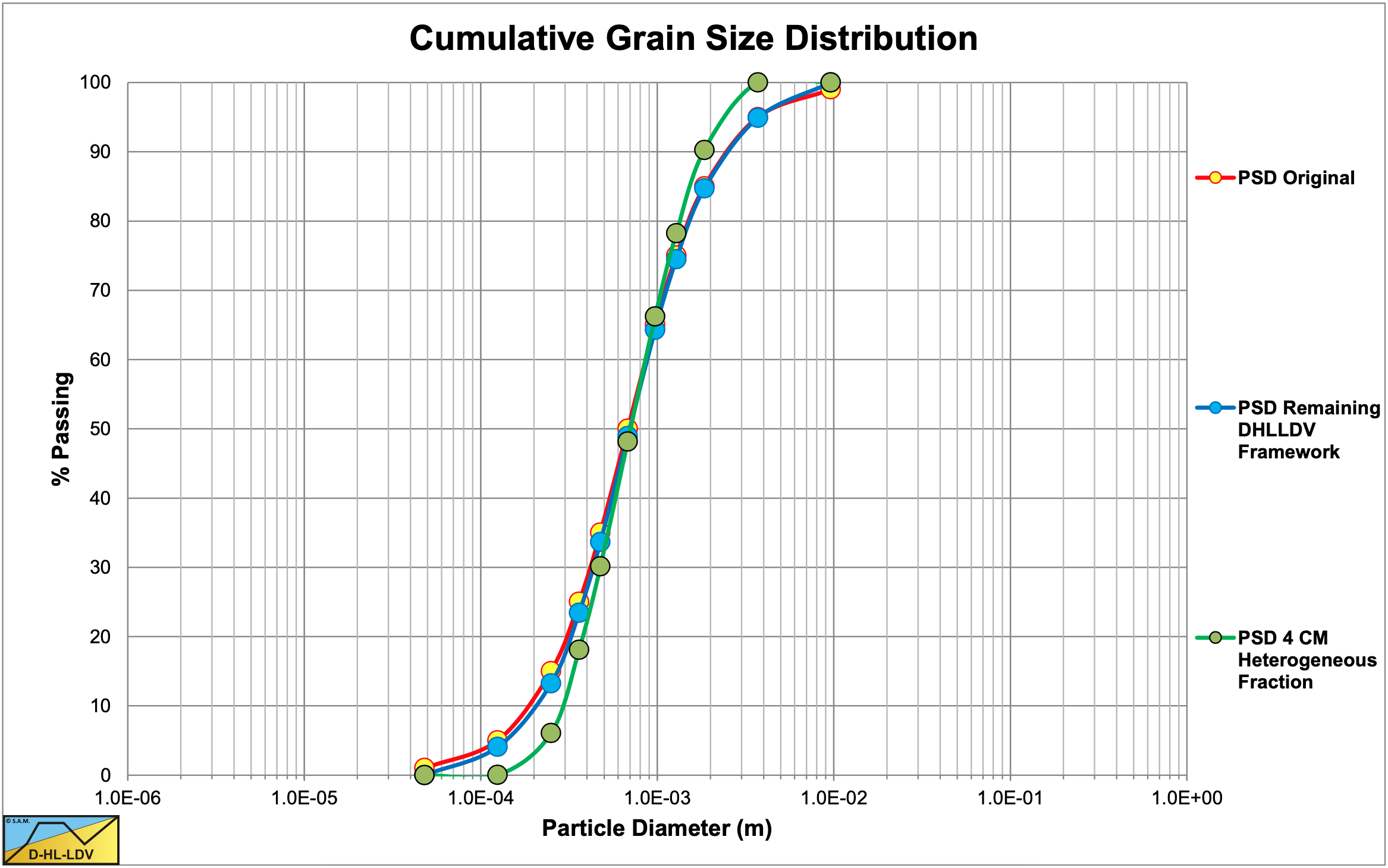
For the original Wilson et al. (2006) model a heterogeneous power M=0.8 is found, while the simplified method gives a power M=1.0. The 4 component model has a power M=1.0.

Figure 6.20-28: The 4 components and the resulting curve.

Figure 6.20-29: The experiments of Clift et al. (1982) versus the 4 component model, the heterogeneous model and the DHLLDV Framework, i_m(v_ls).

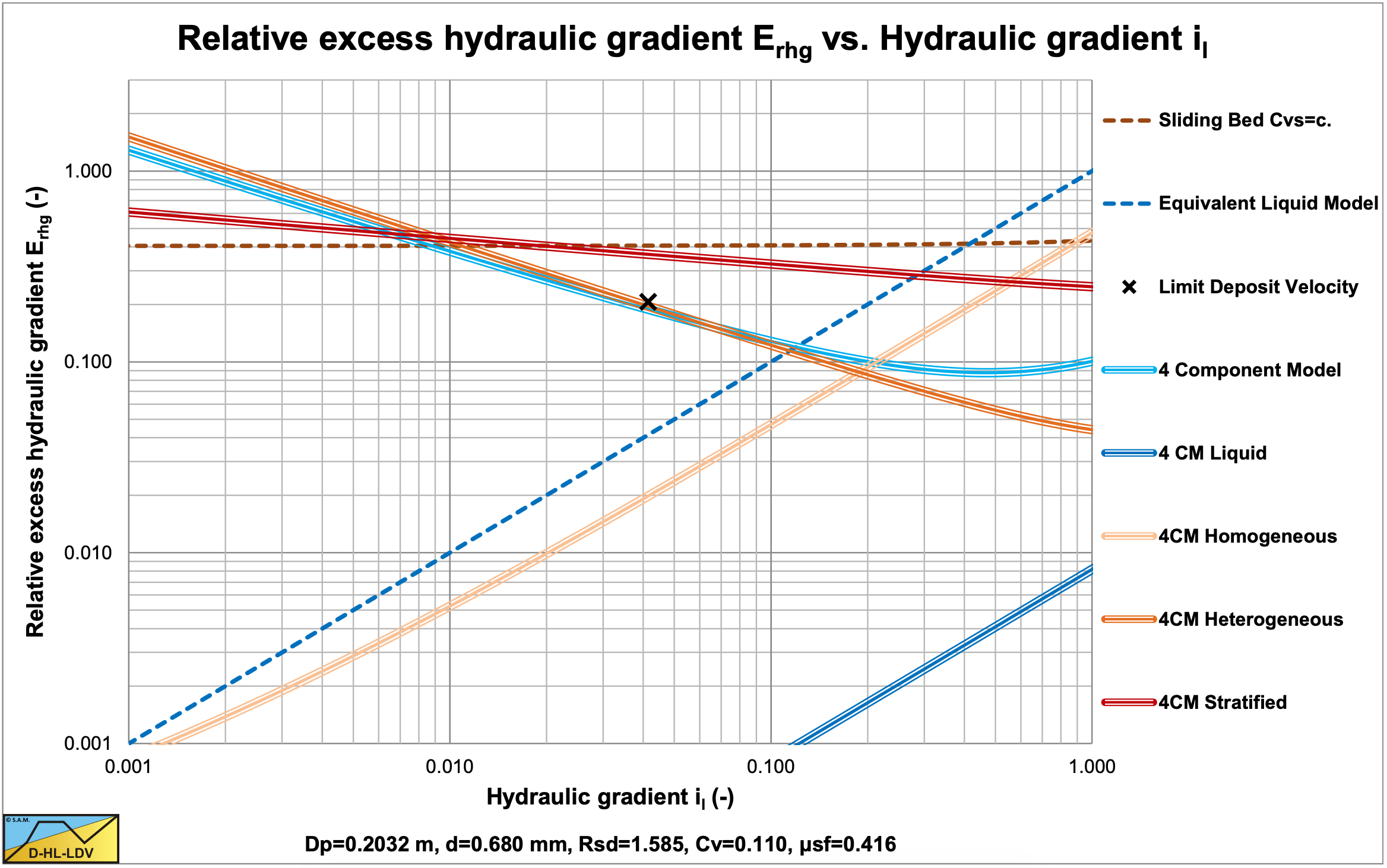
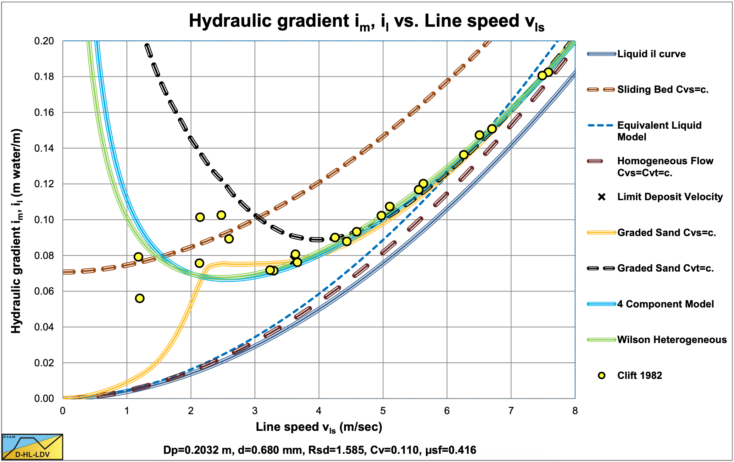
Figure 6.20-28 shows the curves for the 4 components as if each component has the concentration of 11%. The resulting curve is also shown based on the fractions of each component. On the left side the resulting 4CM curve is a bit lower than the heterogeneous curve, since the homogeneous, pseudo homogeneous and the stratified fractions are lower. In the center of the graph the resulting 4CM curve and the heterogeneous curve are almost on top of each other. On the right side the resulting 4CM curve bends upwards because of the increasing values of the homogeneous and pseudo homogeneous curves. Of course this depends on the magnitude of the different fractions.

Figure 6.20-30: The experiments of Clift et al. (1982) versus the 4 component model, the heterogeneous model and the DHLLDV Framework, E_rhg(i_l).

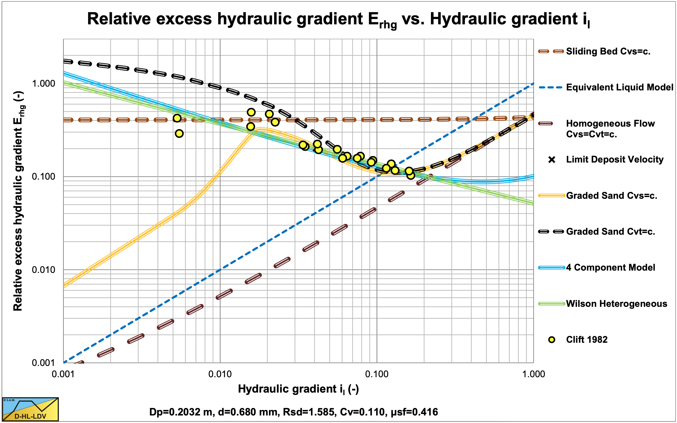
Figure 6.20-29 and Figure 6.20-30 show the data of Clift et al. (1982) versus the 4 component model, the heterogeneous model and the DHLLDV Framework. From personal communication it is known that both the heterogeneous model and the 4 component model are developed for operational conditions, which is above the LDV. The LDV in the case considered is v_ls,ldv=3.63 m/s or i_l=0.04. Above this the models match very well with the experimental data and also with the DHLLDV Framework. It should be mentioned that both the heterogeneous model and the 4 component model do not approach the ELM or the reduced ELM at high line speeds, where the DHLLDV Framework does. The choice of choosing a dh based on the heterogeneous PSD seems to be a good choice, giving a good match with the experimental data.

The grading of the crushed granite is broad, but still the non-heterogeneous fractions are not too large. Reason to investigate a broader graded PSD. Figure 6.20-31 shows the PSD of a very broad graded material with a d₅₀=0.68 mm. The ratio d₈₅/d₅₀=8.154. Now the homogeneous fraction is 8.77%, the pseudo homogeneous fraction 17.90%, the heterogeneous fraction 50.89% and the stratified fraction 22.44%. The d_h=d₅₀=0.63 mm., the v₅₀=3.22 m/s. Because of the larger homogeneous fraction, both the fluid viscosity and density are adjusted.

Figure 6.20-32 shows the curves for the 4 individual components and the resulting 4CM. The homogeneous curve is higher because of a larger homogeneous fraction. The pseudo homogeneous, heterogeneous and stratified fraction curves are not influenced by this. On the left side the curves show upwards curvature. This is because of the higher viscosity due to a larger homogeneous fraction. The heterogeneous curve has the same steepness compared to Figure 6.20-28, however the resulting 4CM curve is less steep.

Figure 6.20-33 and Figure 6.20-34 again compare the experimental data of Clift et al. (1982) with the heterogeneous model, the 4 component model and the DHLLDV Framework. Above v_ls,ldv=3.63 m/s or i_l=0.04 the curves are less steep than the data points, which is expected based on the theory. The 3 models match very well among each other under operational conditions, but deviate both for higher and lower line speeds. At low line speeds the slip (the velocity difference between particles and liquid) increases resulting in plug flow at very low line speeds. This is not covered by the heterogeneous and the 4 component model, since they were derived for operational conditions. Both the heterogeneous and the 4 component model give a hydraulic gradient approaching the pure carrier liquid hydraulic gradient for very high line speeds, and do not follow a reduced ELM model in this case. The DHLLDV Framework covers both very low and very high line speeds and takes the omissions into consideration.

Figure 6.20-31: The PSD of very broad graded granite, reconstructed.

Figure 6.20-32: The 4 components and the resulting curve, very broad graded granite.

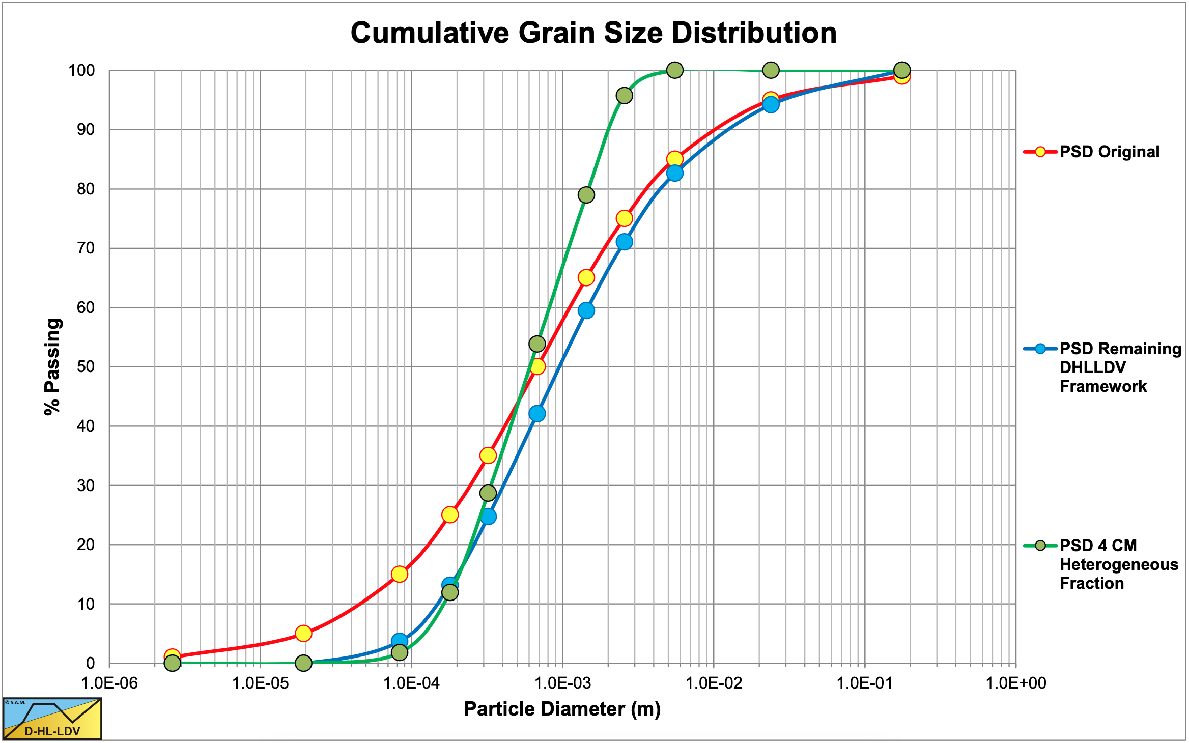
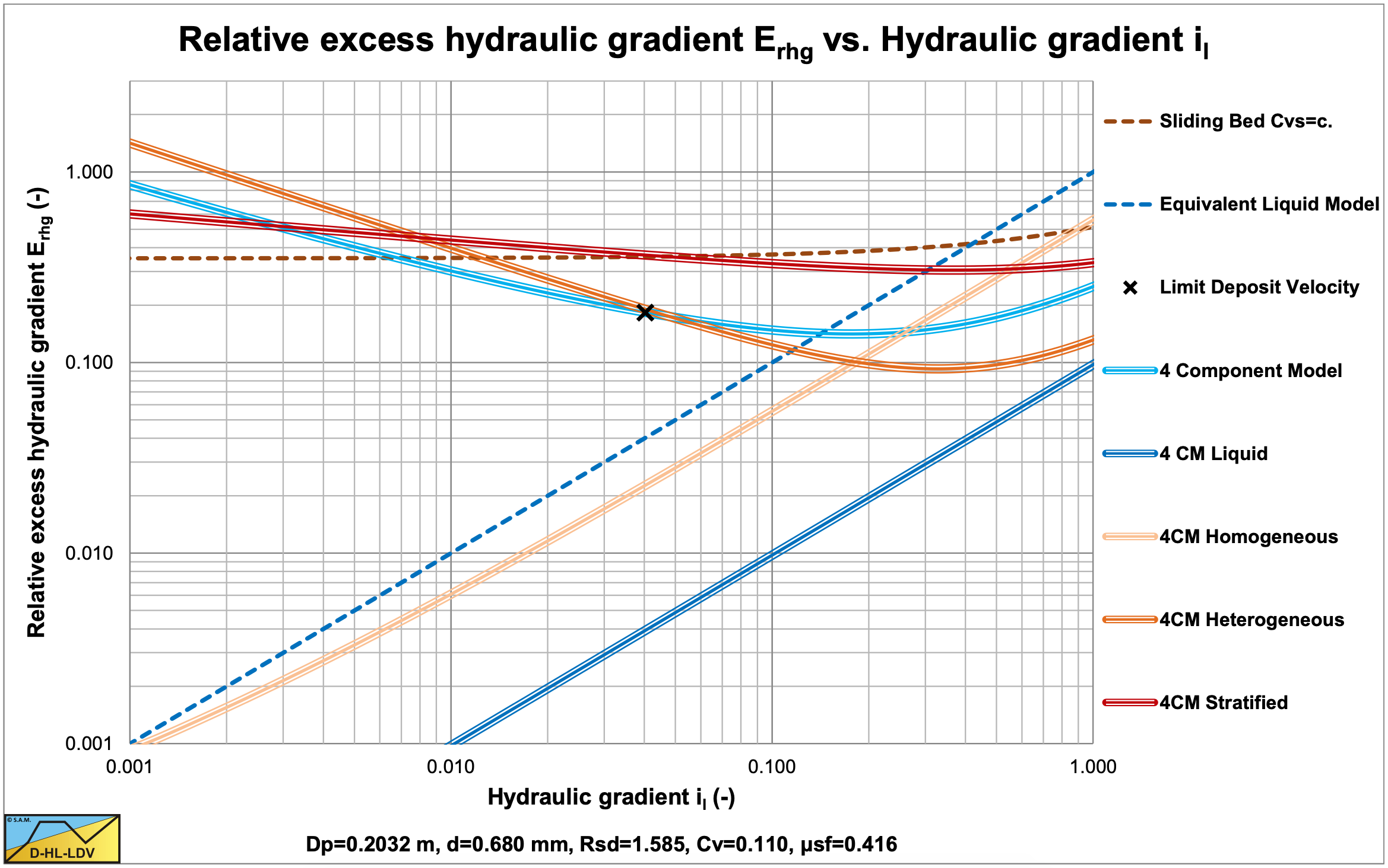
Under operational conditions the difference between the heterogeneous model and the 4 component model seems to be marginal and within the scatter of the experimental data. The 4 component model uses fixed boundaries regarding the 4 components, while these boundaries are most probably line speed dependent. Especially the transition heterogeneous-stratified is line speed dependent.

Figure 6.20-33: The experiments of Clift et al. (1982) versus the 4 component model, the heterogeneous model and the DHLLDV Framework, i_m(v_ls), very broad graded granite.

Figure 6.20-34: The experiments of Clift et al. (1982) versus the 4 component model, the heterogeneous model and the DHLLDV Framework, E_rhg(i_l), very broad graded granite.

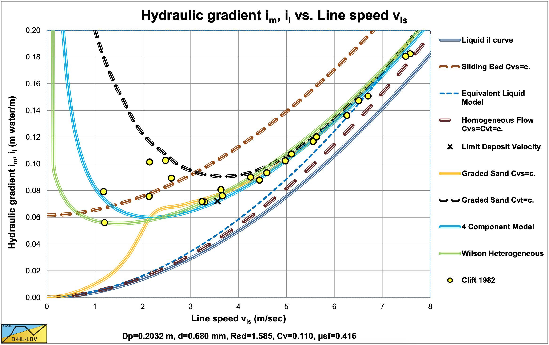
6.20.3.9 Conclusions & Discussion

The 4 component model of Wilson et al. (2006) divides a PSD into 4 fractions, homogeneous, pseudo homogeneous, heterogeneous and stratified. The method assumes these fractions are fixed and do not depend on the line speed (cross-section averaged velocity in the pipe) of the mixture and hardly on the pipe diameter (only the stratified fraction). The different equations for the 4 flow regimes have been derived for line speeds around the working point of a pump pipeline system based on many experiments. For lower or higher line speeds however, the boundaries of the 4 fractions will differ. If the line speed is much lower, part of the heterogeneous fraction (the coarse part) will be stratified since the heterogeneous hydraulic gradient will not be larger than the stratified hydraulic gradient, decreasing the heterogeneous fraction and increasing the stratified fraction. Also part of the pseudo homogeneous fraction may become heterogeneous, reducing the pseudo homogeneous fraction and increasing the heterogeneous fraction. At much higher line speeds the fine part of the heterogeneous fraction will become pseudo homogeneous, while the fine part of the stratified fraction may become heterogeneous. Whether this is relevant for normal dredging practice is the question, but one should realize this. The equations for the homogeneous and pseudo homogeneous flow are clear, although the way the densities are determined seem incorrect. Apparently Wilson et al. (2006) use the definitions for homogeneous flow both the fluid density and viscosity are influenced by the homogeneous fraction, while for pseudo homogeneous flow only the fluid density is influenced by the pseudo homogeneous fraction. The equation for heterogeneous flow raises some questions. Wilson et al. (2006) state that 50% of the solids are stratified, while the other 50% apparently is in suspension at a line speed v₅₀. They also state that the E_rhg parameter at this line speed equals half the friction coefficient, assuming a sliding friction coefficient of μ_sf=0.44, this gives E_rhg=0.22. This implies that the 50% solids in suspension do not contribute to the hydraulic gradient, which is awkward. Now, if the 4 component model is used, this is not an issue, since the homogeneous and pseudo homogeneous fractions are taken into account separately, but in case the heterogeneous model is applied individually this is an issue. The following equation would give a correct hydraulic gradient. This equation is in fact already a 2 component model. Adjusting the liquid properties for the real homogeneous fraction would make it a 3 component model.

\[\ \mathrm{i}_{\mathrm{m}}-\mathrm{i}_{\mathrm{l}}=\mathrm{C}_{\mathrm{v} \mathrm{t}} \cdot \mathrm{R}_{\mathrm{s} \mathrm{d}} \cdot\left(\mu_{\mathrm{s f}} \cdot \frac{\mathrm{1}}{2} \cdot\left(\frac{\mathrm{v}_{\mathrm{5} 0}}{\mathrm{v}_{\mathrm{l s}}}\right)^{\mathrm{M}}+\mathrm{A} \cdot \mathrm{i}_{\mathrm{l}} \cdot\left(\mathrm{1}-\frac{\mathrm{1}}{\mathrm{2}} \cdot\left(\frac{\mathrm{v}_{\mathrm{5} 0}}{\mathrm{v}_{\mathrm{l s}}}\right)^{\mathrm{M}}\right)\right)\]

It is also strange that the hydrostatic approach to determine the normal force on the pipe wall is not applied here. For small spatial volumetric concentrations the multiplication factor is almost 1, but for large concentrations a value of 1.3 can be reached. Maybe this effect is already included in the factor 0.22 and the power M, but this is not clear. If the weight approach of Miedema & Ramsdell (2014) is used, the equation is correct. Another issue is the sliding friction coefficient μ_sf. In the equation for the heterogeneous fraction μ_sf=0.44 is used, while the equation for the stratified fraction uses μ_sf=0.4. The model should be consistent in itself and use one and the same sliding friction coefficient μ_sf, unless there is an explicit reason to use different sliding friction coefficients for different flow regimes. In the equations in this chapter, consequently the symbol for the sliding friction factor μ_sf is used instead of numerical values. Wilson et al. (2006) use the hydrostatic approach to determine the total normal force between the bed and the pipe wall. The result of this is a normal force larger than the weight of the bed. If the bed fills the pipe for 50%, the weight has to be multiplied by 1.3 and for a full pipe with a factor 2. From 0% to 50% this factor increases from 1 to 1.3. In the original equation of Wilson et al. (2006) for stratified flow, the E_rhg value at v_sm equals 2 times the sliding friction coefficient, matching the hydrostatic approach for a full pipe, but not for a partially filled pipe. In the 4 component model it is assumed that stratified fraction is only a limited fraction of the PSD, otherwise the stratified model should be applied. If only a limited fraction is stratified, the multiplication factor of the normal force with respect to the weight of the bed is close to 1. This is probably the reason why Wilson et al. (2006) multiplied their original stratified equation with a factor 0.5, resulting in an E_rhg value at v_sm equal to the sliding friction coefficient μsf. The reason they mention, it’s because of the fines, does not make sense, since they already correct the equation for the relative submerged density of the solids, floating in a mixture of the homogeneous, pseudo homogeneous and heterogeneous fractions. Whether the latter is correct is also the question, since the stratified flow is dominated by the weight of the bed as a whole, resulting in sliding friction. The Wilson et al. (2006) model and their 4 component model are not yet internally consistent and still raise some questions. On the other hand the models are based on numerous experiments and are expected to give reasonable predictions in the neighborhood of the working point of normal dredging operations.

Equation (6.20-95) gives a correction for the fact that the v₅₀ is overestimated for small particles. The original v₅₀ equation gives a constant value for small particles, the simplified equation still overestimates. It would be more convenient to give a better v₅₀ equation, instead of correcting a wrong equation.

6.20.4 Near Wall Lift

Wilson et al. (2000) found that close to the bottom of the pipe the volumetric concentration is lower than just above the bottom of the pipe. They explain this phenomena as the effect of near wall turbulent lift. If there is a strong curvature of the velocity profile, which there is in turbulent flow close to the wall, particles in this flow will be subject to a lift force. This should not be mistaken with Magnus lift in a laminar flow (in the viscous sub-layer). Sellgen and Wilson stated that Matoušek (2006) found from experiments in a vertical 0.15 m-diameter pipeline with narrowly graded sands (Average particle sizes of 0.12, 0.37, 1.84 mm) and concentrations by volume up to about 35% that the medium-sand particles gave less pipe wall friction than both the coarse-sand and fine-sand particles. He discussed various mechanisms and confirmed that the medium-sand particles showed stronger hydrodynamic repelling force off the wall than the others at velocities of practical interest, in accord with theoretical estimations by Wilson & Sellgren (2002).

Wilson et al. (2010) introduced the lift force F_L on a particle as:

\[\ \mathrm{F}_{\mathrm{L}}=\mathrm{C}_{\mathrm{L}} \cdot \frac{\mathrm{1}}{2} \cdot \rho_{\mathrm{l}} \cdot \mathrm{u}_{*}^{\mathrm{2}} \cdot \frac{\pi}{4} \cdot \mathrm{d}^{\mathrm{2}}\]

And for the weight of the particle F_W:

\[\ \mathrm{F}_{\mathrm{W}}=\left(\rho_{\mathrm{s}}-\rho_{\mathrm{l}}\right) \cdot \mathrm{g} \cdot \frac{\pi}{6} \cdot \mathrm{d}^{\mathrm{3}}\]

Giving for the so called lift ratio L_R, the ratio of the lift force on a particle F_L to the weight of a particle F_W:

\[\ \mathrm{L}_{\mathrm{R}}=\frac{\mathrm{F}_{\mathrm{L}}}{\mathrm{F}_{\mathrm{W}}}=\mathrm{C}_{\mathrm{L}} \cdot \frac{\mathrm{3}}{4} \cdot \frac{\mathrm{u}_{*}^{2}}{\mathrm{R}_{\mathrm{s d}} \cdot \mathrm{g} \cdot \mathrm{d}}=\frac{\mathrm{3}}{4} \cdot \mathrm{C}_{\mathrm{L}} \cdot \frac{\rho_{\mathrm{l}} \cdot \mathrm{u}_{*}^{\mathrm{2}}}{\rho_{\mathrm{l}} \cdot \mathrm{R}_{\mathrm{s d}} \cdot \mathrm{g} \cdot \mathrm{d}}=\frac{\mathrm{3}}{4} \cdot \mathrm{C}_{\mathrm{L}} \cdot \theta=\mathrm{C}_{\mathrm{L}} \cdot \frac{\mathrm{3}}{32} \cdot \frac{\lambda_{\mathrm{l}} \cdot \mathrm{v}_{\mathrm{l} \mathrm{s}}^{2}}{\mathrm{R}_{\mathrm{s d}} \cdot \mathrm{g} \cdot \mathrm{d}}\]

With: θ=Shields parameter.

This ratio will be referred to as the lift force to weight ratio or just the lift ratio. If this ratio is bigger than 1, particles will be lifted, otherwise gravity dominates. Now it is the question whether or not the lift force is completely correct, but it can be used as an indication. In Wilson et al. (2006) a lift coefficient C_L=0.27 is mentioned for spheres and not necessarily for sand and granite.

The line speed where the lift ratio equals 1 can now be determined with:

\[\ \mathrm{v}_{\mathrm{ls}, \mathrm{L}_{\mathrm{R}}=1}^{2}=\frac{32}{3} \cdot \frac{\mathrm{R}_{\mathrm{sd}} \cdot \mathrm{g} \cdot \mathrm{d}}{\mathrm{C}_{\mathrm{L}} \cdot \lambda_{\mathrm{l}}} \quad \Rightarrow \quad \mathrm{v}_{\mathrm{ls}, \mathrm{L}_{\mathrm{R}}=1}=\left(\frac{32}{3} \cdot \frac{\mathrm{R}_{\mathrm{sd}} \cdot \mathrm{g} \cdot \mathrm{d}}{\mathrm{C}_{\mathrm{L}} \cdot \lambda_{\mathrm{l}}}\right)^{0.5}\]

Now the idea is that in some circumstances particles will be lifted away from the bottom of the pipe, leaving a particle lean region near the wall, which is in agreement with the concentration profiles found. Medium sized particles show a hydraulic gradient below the ELM curve after passing this curve, see Figure 6.20-35. The asymptotic behavior for very high line speeds cannot be established from the data, since in general experiments are not carried out with very high line speeds, but at line speeds close to operational line speeds or lower. Figure 6.20-36 shows data from Blythe & Czarnotta (1995) also showing crossing the ELM. However these data points seem to return to the ELM at higher line speeds, or at least follow a parallel curve, not approaching the pure liquid behavior.

Based on the so called shear Reynolds number:

\[\ \text{Re}_{*}=\frac{\mathrm{v}_{*} \cdot \mathrm{d}}{v_{\mathrm{l}}}\]

A new expression has been derived for the stratification ratio R:

\[\ \mathrm{E}_{\mathrm{r h g}}=\frac{\mathrm{i}_{\mathrm{m}}-\mathrm{i}_{\mathrm{l}}}{\mathrm{R}_{\mathrm{s d}} \cdot \mathrm{C}_{\mathrm{v t}}}=\mathrm{R}=\frac{\mathrm{0 . 9 3}}{\theta \cdot\left(\mathrm{R} \mathrm{e}_{*}\right)^{1 / 3}}\]

Figure 6.20-35: The data of Whithlock et al. (2004).

Figure 6.20-36: The data of Blythe & Czarnotta (1995).

The coefficient is slightly different from the original paper (0.93 instead of 0.7) because here the Shields parameter is applied. According to Wilson et al. (2010) the stratification ratio has an upper limit of 0.6. The shear velocity used in this Reynolds number is the shear velocity based on the terminal settling velocity of the particle. Now assuming a cylinder around the particle with diameter d and height d, the shear stress on the surface of this cylinder follows from the weight of the particle and the surface of this cylinder, so:

\[\ \begin{array}{left} \tau_{\mathrm{c}} \cdot \pi \cdot \mathrm{d}^{2}=\left(\rho_{\mathrm{s}}-\rho_{\mathrm{l}}\right) \cdot \mathrm{g} \cdot \frac{\pi}{6} \cdot \mathrm{d}^{\mathrm{3}}\\
\tau_{\mathrm{c}}=\left(\rho_{\mathrm{s}}-\rho_{\mathrm{l}}\right) \cdot \mathrm{g} \cdot \frac{\mathrm{1}}{\mathrm{6}} \cdot \mathrm{d}\end{array}\]

Assuming a similar relation between the shear stress and the shear velocity gives:

\[\ \begin{array}{left}\tau_{\mathrm{c}}=\rho_{\mathrm{l}} \cdot \mathrm{v}_{*}^{2}=\left(\rho_{\mathrm{s}}-\rho_{\mathrm{l}}\right) \cdot \mathrm{g} \cdot \frac{1}{6} \cdot \mathrm{d}\\
\mathrm{v}_{*}=\left(\frac{\left(\rho_{\mathrm{s}}-\rho_{\mathrm{l}}\right)}{6 \cdot \rho_{\mathrm{l}}} \cdot \mathrm{g} \cdot \mathrm{d}\right)^{1 / 2}=\left(\frac{\mathrm{R}_{\mathrm{sd}} \cdot \mathrm{g} \cdot \mathrm{d}}{6}\right)^{1 / 2}\\
\operatorname{Re}_{*}=\frac{\mathrm{v}_{*} \cdot \mathrm{d}}{v_{\mathrm{l}}}=\frac{\left(\frac{\mathrm{R}_{\mathrm{sd}} \cdot \mathrm{g} \cdot \mathrm{d}}{6}\right)^{1 / 2} \cdot \mathrm{d}}{v_{\mathrm{l}}}\end{array}\]

Now substituting both the Shields parameter and the shear Reynolds number in the stratification ratio equation gives:

\[\ \begin{array}{left}\mathrm{E}_{\mathrm{rhg}}=\frac{\mathrm{i}_{\mathrm{m}}-\mathrm{i}_{\mathrm{l}}}{\mathrm{R}_{\mathrm{s} \mathrm{d}} \cdot \mathrm{C}_{\mathrm{v t}}}=\mathrm{R}=\frac{\mathrm{0 . 9 3}}{\left(\frac{\lambda_{1} \cdot \mathrm{v}_{\mathrm{l s}}^{2}}{\mathrm{8} \cdot \mathrm{R}_{\mathrm{s d}} \cdot \mathrm{g} \cdot \mathrm{d}}\right) \cdot\left(\frac{\left(\frac{\mathrm{R}_{\mathrm{s d}} \cdot \mathrm{g} \cdot \mathrm{d}}{\mathrm{6}}\right)^{1 / 2} \cdot \mathrm{d}}{v_{\mathrm{l}}}\right)^{1 / 3}}\\
\mathrm{E}_{\mathrm{r h g}}=\mathrm{R}=\frac{\mathrm{1 0} \cdot\left(\mathrm{R}_{\mathrm{s d}} \cdot \mathrm{g} \cdot \mathrm{d}\right)^{1 / 2} \cdot\left(\mathrm{R}_{\mathrm{s} \mathrm{d}} \cdot \mathrm{g} \cdot v_{\mathrm{l}}\right)^{1 / 3}}{\lambda_{1} \cdot \mathrm{v}_{\mathrm{ls}}^{2}}\end{array}\]

With this equation, the proportionality with the line speed is about -1.8. The Shields parameter has a proportionality of 2 because of the line speed squared and about -0.2 because of the Darcy Weisbach friction factor, resulting in a power of -1.8. The shear Reynolds number has a power of 0. So this totals to -1.8, which gives a slightly steeper decrease of the hydraulic gradient or stratification ratio of the original model having a power of -1.7 for uniform PSD’s. The simplified heterogeneous model used:

\[\ \mathrm{E}_{\mathrm{r h g}}=\mathrm{R}=\frac{\mathrm{i}_{\mathrm{m}}-\mathrm{i}_{\mathrm{l}}}{\mathrm{R}_{\mathrm{s} \mathrm{d}} \cdot \mathrm{C}_{\mathrm{v}}}=\frac{\mu_{\mathrm{s} \mathrm{f}}}{2} \cdot\left(\frac{\mathrm{v}_{\mathrm{5} 0}}{\mathrm{v}_{\mathrm{ls}}}\right)^{\mathrm{M}}\]

With:

\[\ \begin{array}{left}\mathrm{v}_{\mathrm{5 0}} \approx \mathrm{3 . 9 3} \cdot\left(\mathrm{1 0 0 0} \cdot \mathrm{d}_{\mathrm{5 0}}\right)^{\mathrm{0 . 3 5}} \cdot\left(\frac{\mathrm{R}_{\mathrm{s d}}}{\mathrm{1 . 6 5}}\right)^{\mathrm{0 . 4 5}} \cdot\left(\frac{v_{\mathrm{l}, \mathrm{a c t u a l}}}{v_{\mathrm{w}, \mathrm{2 0}}}\right)^{-\mathrm{0 . 2 5}}\\
\mathrm{v}_{\mathrm{5 0}} \approx \mathrm{1 . 1 1} \cdot\left(\mathrm{d}_{\mathrm{5 0}}\right)^{\mathrm{0 . 3 5}} \cdot\left(\mathrm{R}_{\mathrm{s d}}\right)^{\mathrm{0 . 4 5}} \cdot\left(v_{\mathrm{l}}\right)^{-\mathrm{0 . 2 5}}\end{array}\]

For sands and gravels this reduces to:

\[\ \mathrm{v}_{\mathrm{5 0}} \approx 44.1 \cdot\left(\mathrm{d}_{\mathrm{5 0}}\right)^{\mathrm{0 . 3 5}}\]

Giving for the simplified equation (with μ_sf=0.44 and M=1.7):

\[\ \mathrm{E}_{\mathrm{rhg}}=\mathrm{R}=\frac{\mu_{\mathrm{sf}}}{2} \cdot\left(\frac{44.1 \cdot\left(\mathrm{d}_{50}\right)^{0.35}}{\mathrm{v}_{\mathrm{l s}}}\right)^{\mathrm{M}}=\mathrm{1 3 7 . 4 \cdot \frac { \mathrm { d } ^ { 0 . 6 } } { \mathrm { v } _ { \mathrm { l } \mathrm { s } } ^ { \mathrm { 1.7 } } }}\]

The near wall lift based equation gives:

\[\ \mathrm{E}_{\mathrm{rhg}}=\mathrm{R}=\frac{\mathrm{d}^{1 / 2}}{\lambda_{\mathrm{l}} \cdot \mathrm{v}_{\mathrm{l} \mathrm{s}}^{2}}\]

For medium sized sand particles in water and large pipe diameters (large flow Reynolds numbers), both equations are close. For example, a 1 mm particle gives a v₅₀ of 3.93 m/s, resulting in R=0.22 according to the simplified method. The near wall lift method results in R=0.20, assuming λ_l=0.01 for large diameter pipes.
In both models the stratification ratio increases with increasing particle diameter and relative submerged density. However the relation of the viscosity is different. The simplified model shows a decreasing stratification ratio with increasing viscosity, while the near wall lift shows the opposite. For sands and gravels in water this will not have a significant influence, but for other solids and liquids it might. The appearance of the Darcy Weisbach friction factor in the denominator of the near wall lift equation results in some dependence of the pipe diameter. The dependence on the sliding friction coefficient is not present anymore in the near wall lift equation.

Using the Shields parameter to explain for the stratification ratio seems interesting however.

6.20.5 Inclined Pipes

Wilson et al. (2006) derived the following equation for heterogeneous transport in horizontal pipes:

\[\ \mathrm{i}_{\mathrm{m}}=\mathrm{i}_{\mathrm{l}}+\frac{\mu_{\mathrm{s f}}}{\mathrm{2}} \cdot\left(\frac{\mathrm{v}_{\mathrm{5 0}}}{\mathrm{v}_{\mathrm{l s}}}\right)^{\mathrm{M}} \cdot \mathrm{R}_{\mathrm{s d}} \cdot \mathrm{C}_{\mathrm{v t}}\]

For inclined pipes they modified the equation, matching the reasoning of Worster & Denny (1955), but with the use of the poser M according to:

\[\ \mathrm{i}_{\mathrm{m}, \mathrm{\theta}}=\mathrm{i}_{\mathrm{l}, \mathrm{\theta}}+\frac{\boldsymbol{\mu}_{\mathrm{s f}}}{\mathrm{2}} \cdot\left(\frac{\mathrm{v}_{\mathrm{5 0}}}{\mathrm{v}_{\mathrm{l s}}}\right)^{\mathrm{M}} \cdot \mathrm{R}_{\mathrm{s d}} \cdot \mathrm{C}_{\mathrm{v t}} \cdot \mathrm{c o s}(\theta)^{\mathrm{M}}+\sin (\theta) \cdot \mathrm{R}_{\mathrm{s d}} \cdot \mathrm{C}_{\mathrm{v t}}\]

The power M has a value of 1.7 for uniform or narrow graded sands and decreases to 0.25 for very broad graded sands. For narrow graded sands the influence of the inclination angle is similar to the Durand & Condolios (1952) and Gibert (1960) approach with a power of 1.5 versus 1.7 for Wilson et al. (2006). For medium graded sands with a power around 1, the influence is similar to the Worster & Denny (1955) approach.

Wilson et al. (2006) use a graph with experimental data for the Deposition Limit. Their Deposition Limit however is the Limit of Stationary Deposit Velocity (LSDV) and not the Limit Deposit Velocity. The LSDV is the line speed where a bed starts sliding, while the LDV is defined in this book as the line speed above which there is no stationary or sliding bed. The LDV is thus always higher than the LSDV. The LSDV does not always exist. For smaller particles it is very well possible that there is a direct transition between the stationary bed regime and the heterogeneous flow regime. The graph used by Wilson et al. (2006) shows an increasing LSDV with increasing inclination angle up to an inclination angle of about 30 degrees above which the LSDV is constant or decreasing. The experimental data stop at an inclination angle of 40 degrees. For negative inclination angles, the LSDV decreases with a decreasing inclination angle. The experimental data stop at an angle of -20 degrees.

6.20.6 The Demi-McDonald of Wilson (1979)

The LSDV of Wilson (1979) based on the 2 layer model was originally given as a nomographic chart, made with the help of Professor F.M. Woods. This nomographic chart is known as the demi-McDonald, because of the shape of the particle diameter curve. Nowadays the fit function equation (6.20-34) is often used.

Figure 6.20-37: The demi-McDonald of Wilson (1979).

Figure 6.20-37 shows the demi-McDonald of Wilson (1979). The figure shows an example of the LSDV for a D_p=0.25 m diameter pipe and a d=1 mm diameter particle. For solids with a density of ρ_s=2.65 ton/m³ like sands and gravels, this gives an LSDV of about 3.1 m/s according to the left part of the nomogram. The right part shows that solids with a density of ρ_s=7.85 ton/m³ like iron, give an LSDV of about 6.5 m/s.

The maximum Limit of Stationary Deposit Velocity (LSDV) v_sm can be estimated by (Matousek (2004)), with d in mm and D_p in m:

\[\ \mathrm{v}_{\mathrm{s m}}=\frac{\mathrm{8 .8 } \cdot\left(\frac{\mu_{\mathrm{s f}} \cdot \mathrm{R}_{\mathrm{s d}}}{\mathrm{0 . 6 6}}\right)^{\mathrm{0 . 5 5}} \cdot \mathrm{D}_{\mathrm{p}}^{\mathrm{0 . 7}} \cdot \mathrm{d}^{\mathrm{1 . 7 5}}}{\mathrm{d}^{\mathrm{2}}{+\mathrm{0 . 1 1} \cdot \mathrm{D}_{\mathrm{p}}^{\mathrm{0 . 7}}}} \quad\text{ and }\quad \mathrm{F}_{\mathrm{L}}=\frac{\mathrm{v}_{\mathrm{S m}}}{\sqrt{\mathrm{2 \cdot g \cdot R}_{\mathrm{s d}} \cdot \mathrm{D}_{\mathrm{p}}}}\]

6.20.7 The Sliding Bed Regime New Developments

Based on the developments of the DHLLDV Framework a new equation has been derived for slip ratio in the sliding bed regime. This equation assumes a sliding bed with sheet flow at the top. Suspension is not taken into account. The equation is derived from many fundamental simulations based on the equilibrium equations of the forces on a sliding bed. Based on the results of these simulations an empirical equation is derived. This empirical equation gives the slip ratio as a function of the relative volumetric concentration, the pipe diameter, the sliding friction coefficient, the LSDV and the line speed. The full equation is equation (7.4-93). Here only the slip ratio at the LSDV is determined.

First of all the relation between the spatial and the delivered concentration can be determined by, based on the slip ratio:

\[\ \mathrm{C}_{\mathrm{v s}}=\left(\frac{\mathrm{v}_{\mathrm{l s}}}{\mathrm{v}_{\mathrm{l s}}-\mathrm{v}_{\mathrm{s l}}}\right) \cdot \mathrm{C}_{\mathrm{v t}}=\left(\frac{\mathrm{1}}{\mathrm{1 - \xi}}\right) \cdot \mathrm{C}_{\mathrm{v t}}\]

The slip ratio at the LSDV from Figure 7.4-33 can be estimated by the following empirical equation:

\[\ \begin{array}{left} \mathrm{C}_{\mathrm{v r}}=\frac{\mathrm{C}_{\mathrm{v} \mathrm{t}}}{\mathrm{C}_{\mathrm{v} \mathrm{b}}}\\
\left.\xi_{\mathrm{l} \mathrm{d} \mathrm{v}}=\left(\mathrm{1}-\mathrm{C}_{\mathrm{v r}}\right) \cdot \mathrm{e}^{\left(-\left(\mathrm{0} . \mathrm{8} \mathrm{3}+\frac{\mu_{\mathrm{sf}}}{4}+\left(\mathrm{C}_{\mathrm{v r}}-\mathrm{0 . 5}\right)^{2}+0.02 \mathrm{5} \cdot \mathrm{D}_{\mathrm{p}}\right) \cdot \mathrm{D}_{\mathrm{p}}^{0.025} \cdot \mathrm{C}_{\mathrm{vr}}^{0.65}\right.}\right)\end{array}\]

For the delivered concentration in the above equation, the delivered concentration of all the particles in the heterogeneous and the sliding bed regimes is taken, in case of a very graded sand or gravel. Now knowing the slip ratio, the spatial volumetric concentration can be determined at the LSDV (v_sm) and with this the approximation equation for the sliding bed hydraulic gradient according to:

\[\ \mathrm{i}_{\mathrm{m}}=\mathrm{i}_{\mathrm{l}}+\frac{\mathrm{C}_{\mathrm{v} \mathrm{s}}\left(\mathrm{v}_{\mathrm{s} \mathrm{m}}\right)}{\mathrm{C}_{\mathrm{vt}}} \cdot \mathrm{C}_{\mathrm{v} \mathrm{t}} \cdot \mathrm{R}_{\mathrm{s} \mathrm{d}} \cdot \mu_{\mathrm{s f}} \cdot\left(\frac{\mathrm{v}_{\mathrm{s m}}}{\mathrm{v}_{\mathrm{ls}}}\right)^{\mathrm{0 . 2 5}}=\mathrm{i}_{\mathrm{l}}+\mathrm{C}_{\mathrm{v} \mathrm{t}} \cdot \mathrm{R}_{\mathrm{s d}} \cdot \mu_{\mathrm{s f}} \cdot\left(\left(\frac{\mathrm{1}}{\mathrm{1}-\xi_{\mathrm{l s d v}}}\right) \cdot\left(\frac{\mathrm{v}_{\mathrm{s m}}}{\mathrm{v}_{\mathrm{l} \mathrm{s}}}\right)^{\mathrm{0 . 2 5}}\right)\]

This methodology would also be a good addition to the 4 component model, for the stratified fraction, using C_vt,h+C_vt,s for the determination of the relative concentration C_vr. The homogeneous and pseudo homogeneous fractions are assumed not to have slip. Wilson et al. (2006) do mention that the second term on the right hand side has to be multiplied with some factor, but how to determine this factor is not clear. By using the slip ratio at the LSDV a good quantification of this factor is achieved. The decreasing slip ratio with increasing line speed is quantified with the (v_sm/v_ls)^0.25 term. This will give good results close to the LSDV. At high line speeds the hydraulic gradient will decrease faster. At very low line speeds the hydraulic gradient is limited to (plug flow):

\[\ \mathrm{i}_{\mathrm{m}}=\mathrm{i}_{\mathrm{l}}+\mathrm{C}_{\mathrm{v} \mathrm{b}} \cdot \mathrm{R}_{\mathrm{s} \mathrm{d}} \cdot \mu_{\mathrm{s} \mathrm{f}}\]

6.20.8 Nomenclature Wilson-GIW Models

Ap	Cross section pipe	m^2
A1	Cross section above bed	m^2
A2	Cross section bed	m^2
Cvb	Volumetric spatial bed concentration	-
Cvc	Spatial volumetric concentration contact load	-
Cvs	Spatial volumetric concentration	-
Cvs,1	Spatial volumetric concentration in cross section 1	-
Cvs,2	Spatial volumetric concentration in cross section 2	-
Cvs,f	Spatial volumetric concentration homogeneous fraction	-
Cvr	Relative volumetric concentration Cvr=Cvs/Cvb	-
Cvr,max	Relative volumetric concentration at maximum LSDV	-
Cvt	Delivered (transport) volumetric concentration	-
Cvt,f	Delivered (transport) volumetric concentration homogeneous fraction	-
Cvt,ph	Delivered (transport) volumetric concentration pseudo homogeneous fraction	-
Cvt,h	Delivered (transport) volumetric concentration heterogeneous fraction	-
Cvt,s	Delivered (transport) volumetric concentration stratified fraction	-
d	Particle diameter	m
d50	Particle diameter with 50% passing	m
DH	Hydraulic diameter	m
Dp	Pipe diameter	m
Erhg	Relative excess hydraulic gradient	-
f	Correction factor heterogeneous flow regime	-
F	Force	kN
F1,l	Force between liquid and pipe wall	kN
F12,l	Force between liquid and bed	kN
F2,pr	Force on bed due to pressure	kN
F2,sf	Force on bed due to friction	kN
F2,l	Force on bed due to pore liquid	kN
Fn	Normal force	kN
Fw	Weight of bed	kN
Fsf	Friction force, sliding	kN
Fr	Froude number	-
g	Gravitational constant 9.81 m/s^2	m/s^2
ibed	Hydraulic gradient sliding bed	m/m
ihom	Hydraulic gradient homogeneous flow	m/m
il	Hydraulic gradient liquid	m/m
im	Hydraulic gradient mixture	m/m
iplug	Hydraulic gradient plug flow	m/m
if	Hydraulic gradient homogeneous fraction	m/m
iph	Hydraulic gradient pseudo homogeneous fraction	m/m
ih	Hydraulic gradient heterogeneous fraction	m/m
is	Hydraulic gradient stratified fraction	m/m
ks	Bed roughness	m
ΔL	Length of pipe section	m
LDV	Limit Deposit Velocity	m/s
LSDV	Limit of Stationary Deposit Velocity	m/s
M	Power stratification ratio between 0.25 and 1.7	-
n	Porosity bed	-
Op	Circumference pipe	m
O1	Circumference pipe above bed	m
O2 ​​​​​​​	Circumference pipe in bed	m
O12	Width of bed	m
Δp	Pressure difference	kPa
Δp1 ​​​​​​​	Pressure difference on cross section 1	kPa
Δp2 ​​​​​​​	Pressure difference on cross section 2	kPa
Δpl ​​​​​​​	Pressure difference liquid	kPa
Δpm ​​​​​​​	Pressure difference mixture	kPa
Δpf	Pressure difference homogeneous fluid	kPa
q	Power to determine the normalised excess hydraulic gradient	-
Re	Reynolds number	-
Rsd	Relative submerged density	-
R	Stratification ratio	-
RH	Hydraulic radius	m
Sf	Relative density homogeneous fraction + carrier liquid	-
Sfp	Relative density homogeneous & pseudo homogeneous fractions + carrier liquid	-
Sfph	Relative density homogeneous & pseudo homogeneous & heterogeneous fractions + carrier liquid	-
Sfphs	Relative density homogeneous & pseudo homogeneous & heterogeneous & stratified fractions + carrier liquid	-
Sm	Relative density mixture	-
Ss	Relative density solids	-
u*	Friction velocity	m/s
v	Velocity	m/s
vs ​​​​​​​	Limit of Stationary Deposit Velocity	m/s
vt ​​​​​​​	Terminal settling velocity	m/s
vt*	Terminal settling velocity where d=0.015·Dp	m/s
vu	Threshold velocity	m/s
vls	Line speed	m/s
vls*	Line speed of intersection sliding bed-heterogeneous where d=0.015·Dp	m/s
v1, v1,m, vr	Cross section averaged velocity above bed	m/s
v2, v2,m, vb	Cross section averaged velocity bed	m/s
vsm	Maximum Limit of Stationary Deposit Velocity (LSDV)	m/s
v50	Line speed with 50% stratification	m/s
v50,min	Line speed with 50% stratification for very fine particles	m/s
v50*	Line speed with 50% stratification where d=0.015·Dp	m/s
v85	Line speed with 85% stratification	m/s
vr	Relative line speed vr=vls/vsm	-
w50	Particle associated velocity matching the d50	m/s
w85	Particle associated velocity matching the d85	m/s
X	Fraction in general	-
Xf	Homogeneous fraction	-
Xph	Pseudo homogeneous fraction	-
Xh	Heterogeneous fraction	-
Xs	Stratified fraction	-
yb	Height of bed	m
α	Multiplication factor bed friction	-
α	Power to determine LSDV	-
β	Power to determine LSDV	-
β	Bed angle	rad
ε	Pipe wall roughness	m
ρl	Density carrier liquid	ton/m^3
ρs	Density solids	ton/m^3
ρm	Mixture density	ton/m^3
ρx	Density mixture with fraction X	ton/m^3
ρf	Density homogeneous fluid	ton/m^3
ρfp	Density homogeneous+pseudo homogeneous fluid	ton/m^3
ρfph	Density homogeneous+pseudo homogeneous+heterogeneous fluid	ton/m^3
ρfphs	Density homogeneous+pseudo homogeneous+heterogeneous+stratified fluid	ton/m^3
θ	Shields parameter	-
θc	Critical Shields parameter	-
λ	Darcy-Weisbach friction factor	-
λl	Darcy-Weisbach friction factor liquid-pipe wall	-
λ1	Darcy-Weisbach friction factor with pipe wall	-
λ2	Darcy-Weisbach friction factor with pipe wall, liquid in bed	-
λ12	Darcy-Weisbach friction factor on the bed	-
λf	Darcy-Weisbach friction factor based on homogeneous fluid properties	-
\(\ v_{\mathrm{l}}\)	Kinematic viscosity	m^2/s
\(\ v_{\mathrm{l,actual}} \)	Actual kinematic viscosity liquid	m^2/s
\(\ v_{\mathrm{W}, \mathrm{2 0}}\)	Kinematic viscosity of water at 20 degrees centigrade	m^2/s
\(\ v_{ \mathrm{f}}\)	Kinematic viscosity homogeneous fluid	m^2/s
\(\ \tau\)	Shear stress	kPa
\(\ \mathrm{\tau}_{\mathrm{l}}\)	Shear stress liquid-pipe wall	kPa
\(\ \tau_{1,\mathrm{l}}\)	Shear stress liquid-pipe wall above bed	kPa
\(\ \tau_{ 12,\mathrm{l}}\)	Shear stress bed-liquid	kPa
\(\ \tau_{ 2,\mathrm{l}}\)	Shear stress liquid-pipe in bed	kPa
\(\ \tau_{ 2,\mathrm{sf}}\)	Shear stress from sliding friction	kPa
μsf	Sliding friction coefficient	-
μl	Dynamic viscosity liquid	Pa·s
μf	Dynamic viscosity homogeneous fluid	Pa·s
μr	Relative dynamic viscosity	-
σn	Normal stress	kPa
ζ	Normalized excess hydraulic gradient	-
ζ∞	Normalized excess hydraulic gradient at infinite line speed	-