6.18: The Fuhrboter (1961) Model

Fuhrboter (1961) in his PhD thesis, collected data on frictional head loss for slurry flow conditions in a D_p=300 mm laboratory pipeline with sand and gravel with particle diameters ranging from d₅₀=0.18 mm to d₅₀=4.6 mm. His starting points were the research of Durand & Condolios (1952) and Silin et al. (1958) and the assumption that the pressure losses depend on the spatial volumetric concentration. A relation between pressure losses and delivered volumetric concentration depends on the relation between the spatial and the delivered volumetric concentrations. Fuhrboter (1961) defined the Limit Deposit Velocity or often called critical velocity as the velocity above which no stationary or sliding bed will occur. This is the same definition as used by Durand & Condolios (1952), but different from Wilson et al. (1992) who uses the transition velocity between a fixed or stationary bed and a sliding bed as the critical velocity. Fuhrboter (1961) reports in detail about the experiments regarding the Limit Deposit Velocity for sands with d₅₀ of 0.18 mm, 0.26 mm, 0.44 mm and 0.83 mm and regarding the pressure losses for sands with d₅₀ of 0.26 mm, 0.44 mm and 0.83 mm, based on spatial volumetric concentrations.

Figure 6.7-1: The data of Fuhrboter with a d50=0.26 mm sand.

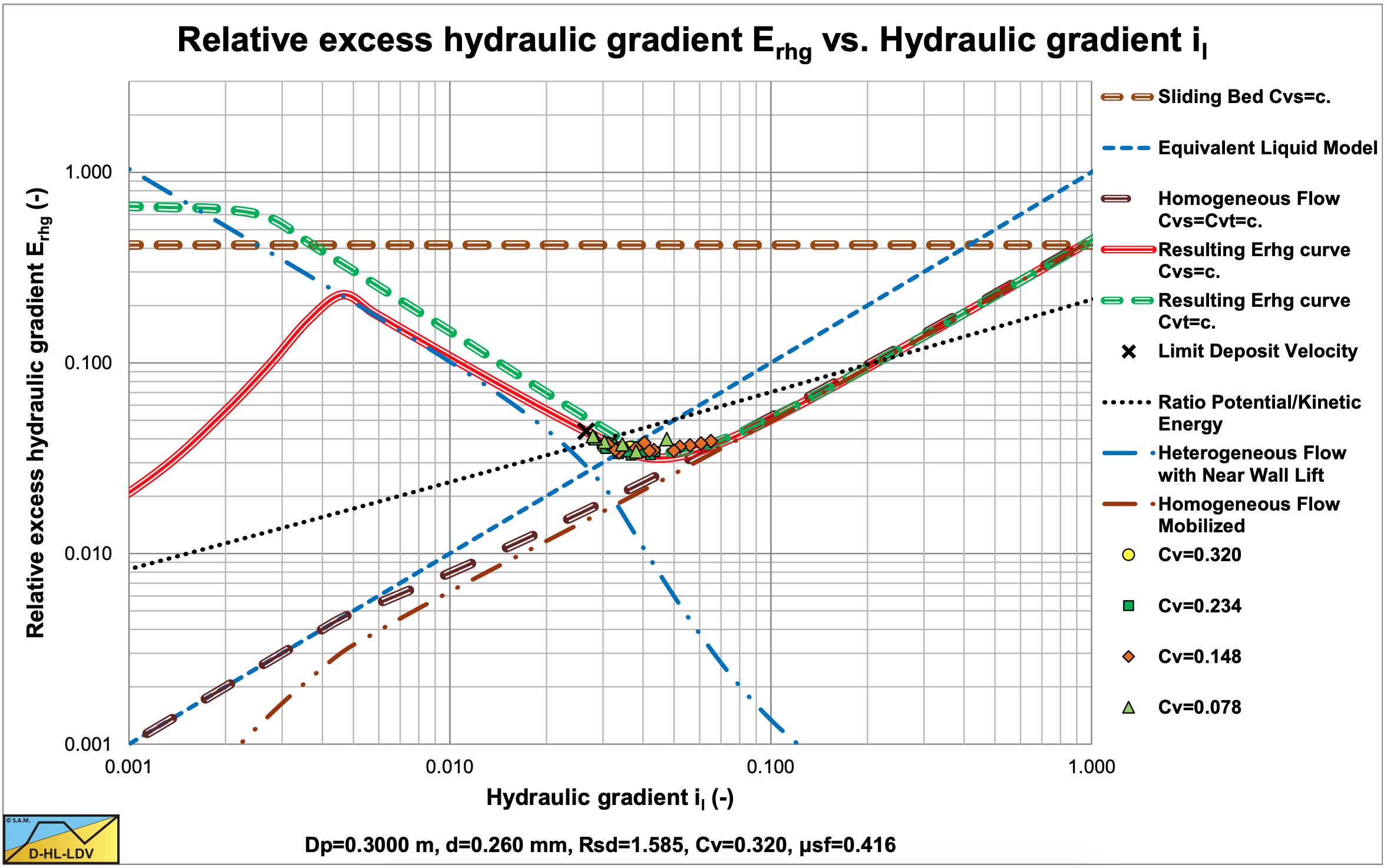
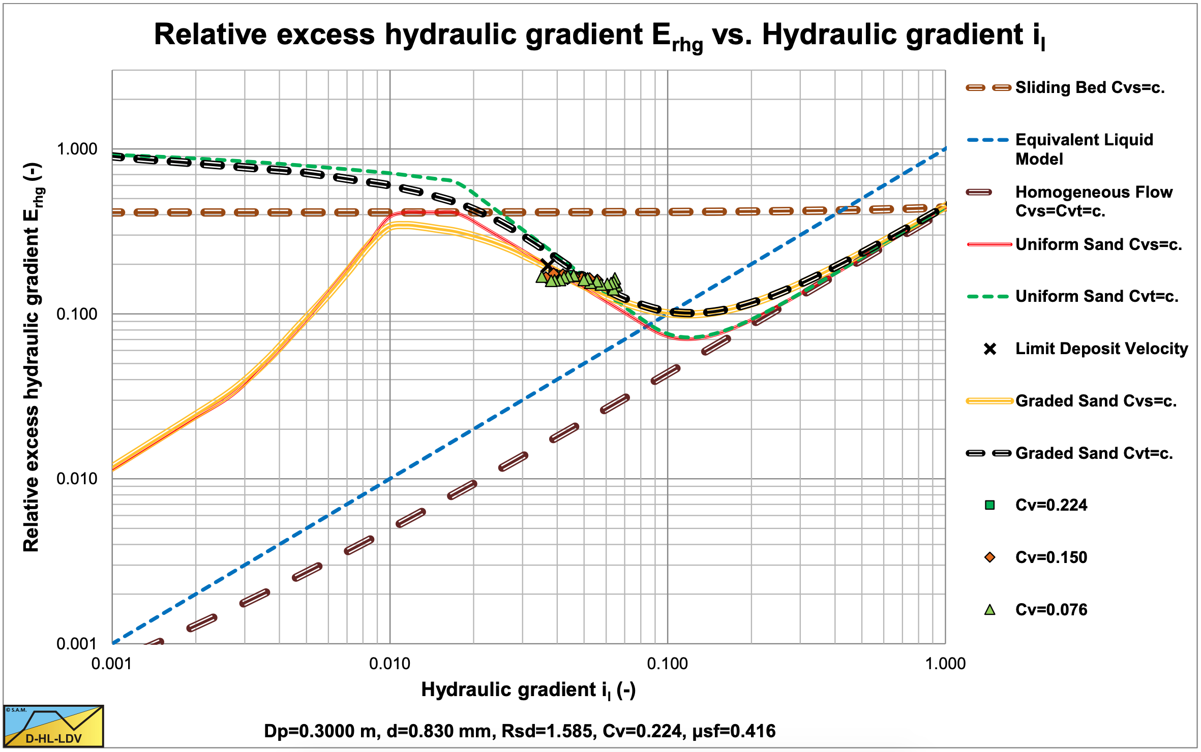
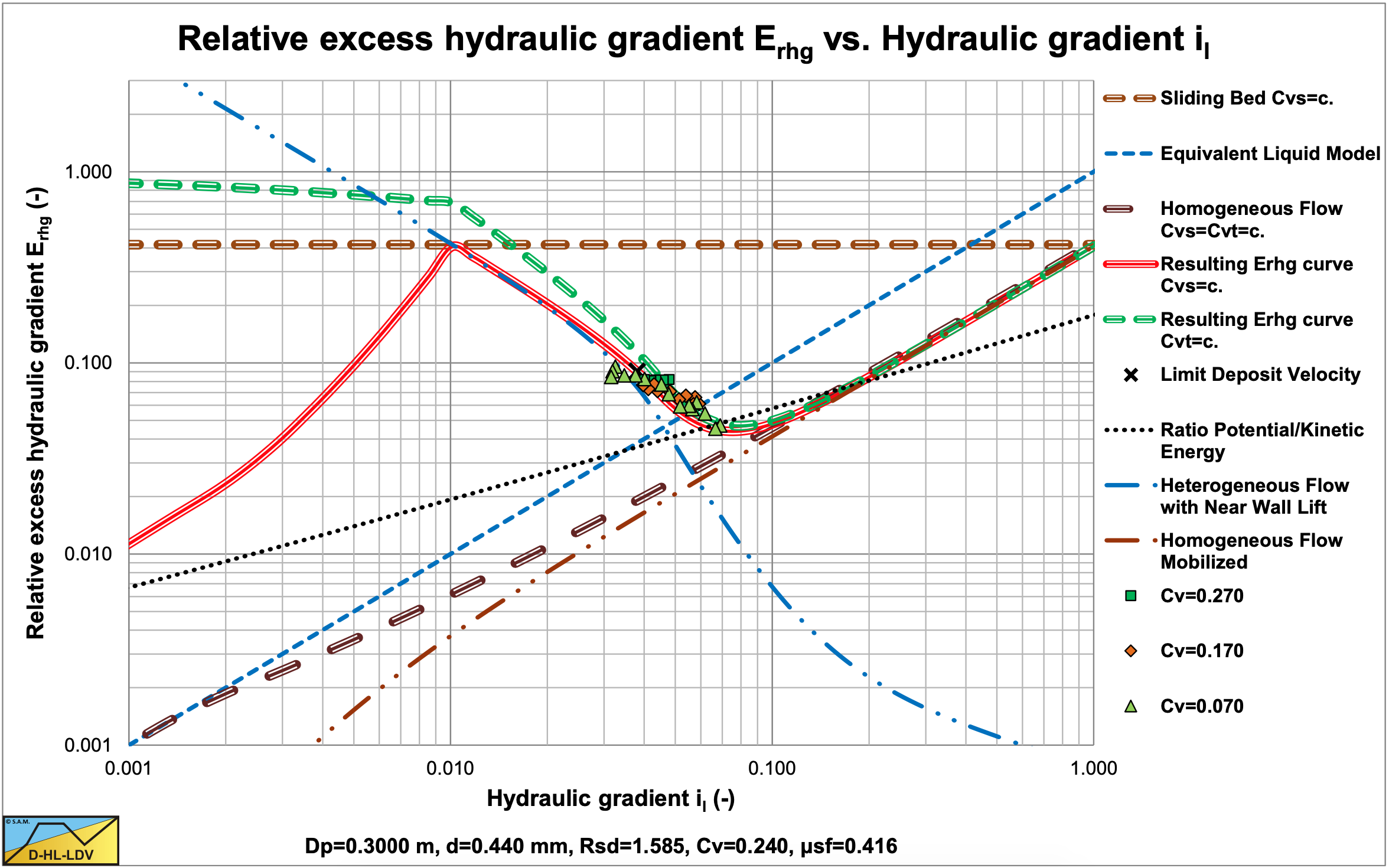
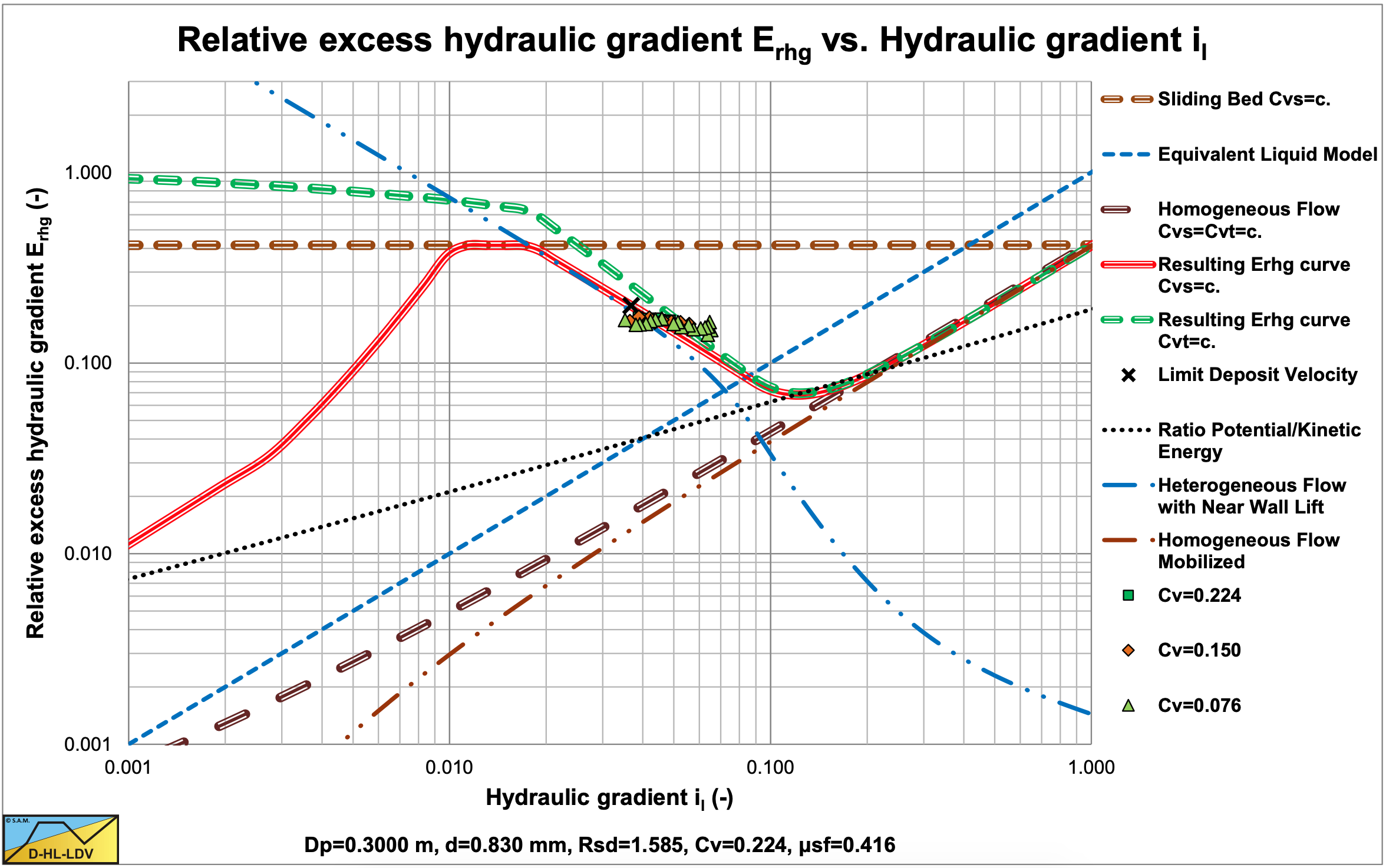
Figure 6.7-1, Figure 6.7-2 and Figure 6.7-3 show the E_rhg values of Fuhrboter for the d₅₀=0.26 mm, d₅₀=0.44 mm and d₅₀=0.83 mm sands, with:

\[\ \mathrm{E}_{\mathrm{rhg}}=\frac{\mathrm{i}_{\mathrm{m}}-\mathrm{i}_{\mathrm{l}}}{\mathrm{R}_{\mathrm{s d}} \cdot \mathrm{C}_{\mathrm{v s}}}\]

The figures show clearly that the experiments were carried out in the heterogeneous flow regime, or at the transition between the heterogeneous and the homogeneous flow regimes for small particles. The data in these figures are only the data points above the Limit Deposit Velocity, giving heterogeneous transport. The heterogeneous curves are based on the original Miedema & Ramsdell (2013) equation. The figures also show the ratio between the potential energy losses and the kinetic energy losses, which is small (<10%) for medium and coarse sands.

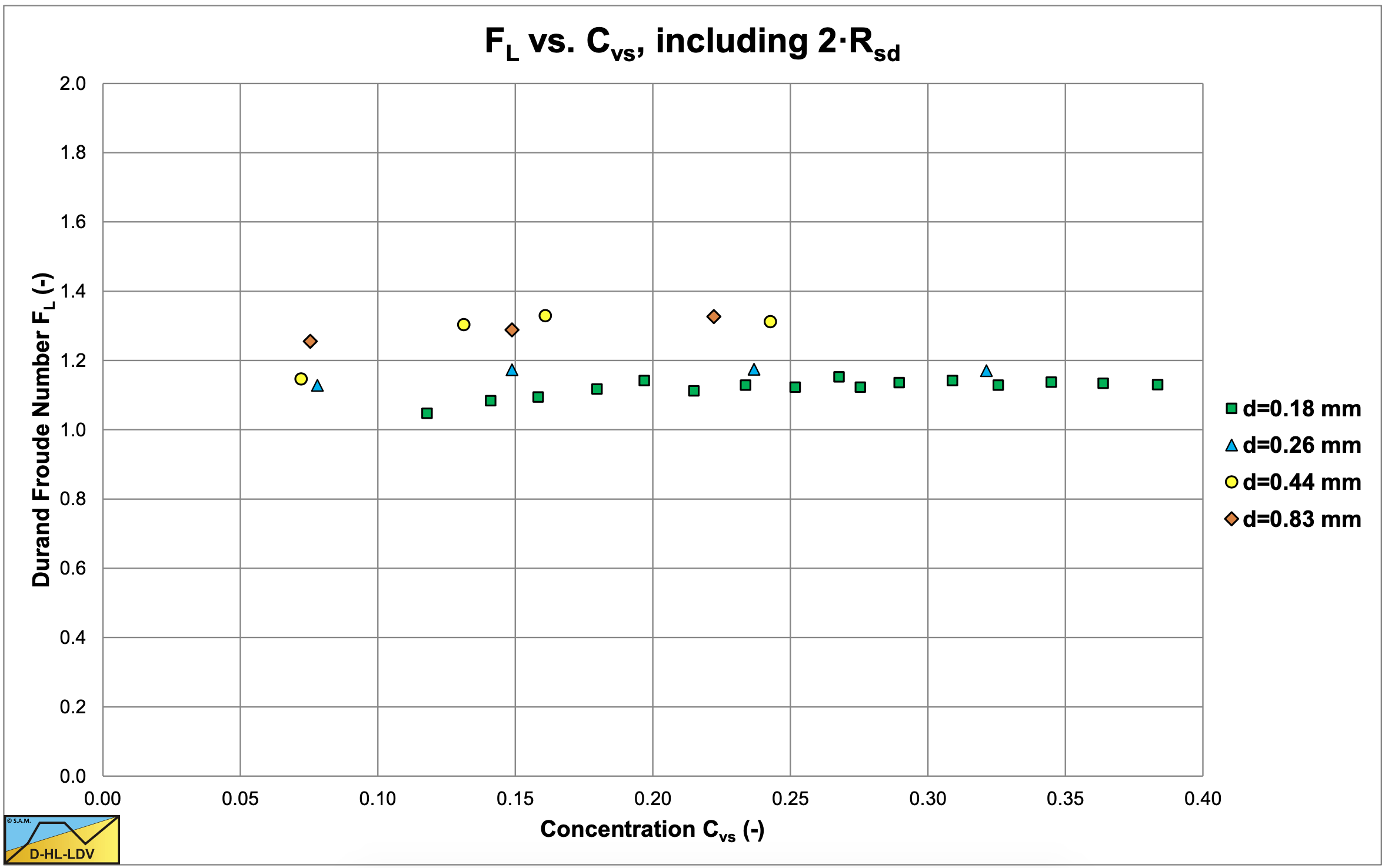
Figure 6.7-4 shows the Durand F_L values for the Limit Deposit Velocity as measured by Fuhrboter, with:

\[\ \mathrm{F}_{\mathrm{L}}=\frac{\mathrm{v}_{\mathrm{l s}, \mathrm{ld v}}}{\sqrt{\mathrm{2 \cdot g} \cdot \mathrm{R}_{\mathrm{s d}} \cdot \mathrm{D}_{\mathrm{p}}}}\]

The data in these figures are only the data points above the Limit Deposit Velocity, giving heterogeneous transport. Based on his findings with heterogeneous transport he proposed the following equation for the frictional head loss:

\[\ \Delta \mathrm{p}_{\mathrm{m}}=\Delta \mathrm{p}_{\mathrm{l}}+\rho_{\mathrm{l}} \cdot \mathrm{g} \cdot \Delta \mathrm{L} \cdot \frac{\mathrm{S}_{\mathrm{k}}}{\mathrm{v}_{\mathrm{l} \mathrm{s}}} \cdot \mathrm{C}_{\mathrm{v} \mathrm{s}}\]

Fuhrboter (1961) separated the excess pressure losses resulting from the solids from the liquid pressure losses, just like Wilson et al. (1992), but different from Durand & Condolios (1952), Jufin & Lopatin (1966) and Newitt et al. (1955) who used:

\[\ \Delta \mathrm{p}_{\mathrm{m}}=\Delta \mathrm{p}_{\mathrm{l}} \cdot\left(\mathrm{1}+\phi \cdot \mathrm{C}_{\mathrm{v}}\right)\]

This results in liquid hydraulic gradients independent excess pressure losses in the Fuhrboter (1961) equation.

Figure 6.7-2: The data of Fuhrboter with a d₅₀=0.44 mm sand.

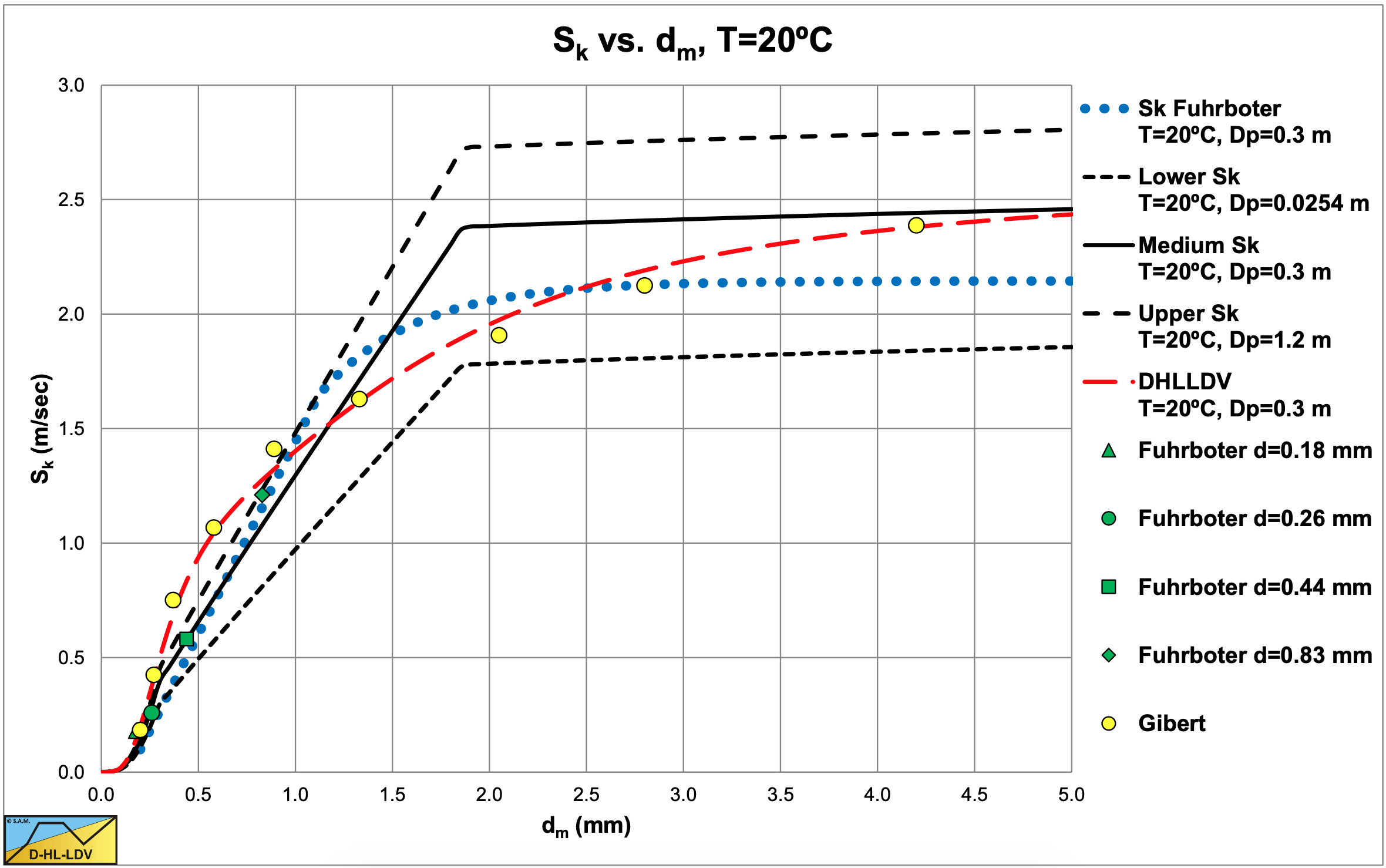
Fuhrboter (1961) did not give an equation for the S_k factor, but showed a graph, which is reproduced in Figure 6.7-5. The concentration C_vs in his equation is the spatial sand concentration and not the delivered volumetric solids concentration C_vt (solely the quarts).
In practice the delivered volumetric solids concentration C_vt is often used. Based on the propagation velocity of density waves/fluctuations, Fuhrboter (1961) concluded that the velocity of the solids was about 65% (+/- 5%) of the flow velocity of the mixture. The factor 0.65 in fact means a slip factor of 0.65 according to Fuhrboter. Fuhrboter modified equation (6.7-3) to equation (6.7-6), applying the fixed slip of 35%, which of course is questionable.

\[\ \mathrm{C}_{\mathrm{v} \mathrm{t}}=\mathrm{0 . 6 5} \cdot \mathrm{C}_{\mathrm{v s}} \quad \Rightarrow \quad \mathrm{S}_{\mathrm{k t}}=\frac{\mathrm{C}_{\mathrm{v s}}}{\mathrm{C}_{\mathrm{v t}}} \cdot \mathrm{S}_{\mathrm{k}} \quad \Rightarrow \quad \mathrm{S}_{\mathrm{k t}}=\frac{\mathrm{1}}{\mathrm{0 . 6 5}} \cdot \mathrm{S}_{\mathrm{k}}\]

\[\ \Delta \mathrm{p}_{\mathrm{m}}=\Delta \mathrm{p}_{\mathrm{l}}+\rho_{\mathrm{l}} \cdot \mathrm{g} \cdot \Delta \mathrm{L} \cdot \frac{\mathrm{S}_{\mathrm{k} \mathrm{t}}}{\mathrm{v}_{\mathrm{l} \mathrm{s}}} \cdot \mathrm{C}_{\mathrm{v t}} \quad\text{ or }\quad \mathrm{i}_{\mathrm{m}}=\mathrm{i}_{\mathrm{l}}+\frac{\mathrm{S}_{\mathrm{k t}}}{\mathrm{v}_{\mathrm{l} \mathrm{s}}} \cdot \mathrm{C}_{\mathrm{v} \mathrm{t}}\]

Figure 6.7-3: The data of Fuhrboter with a d₅₀=0.83 mm sand.

Figure 6.7-4: The Durand F_L factor measured by Fuhrboter.

Figure 6.7-5: The transport factor S_k and S_kt for the Fuhrboter equation.

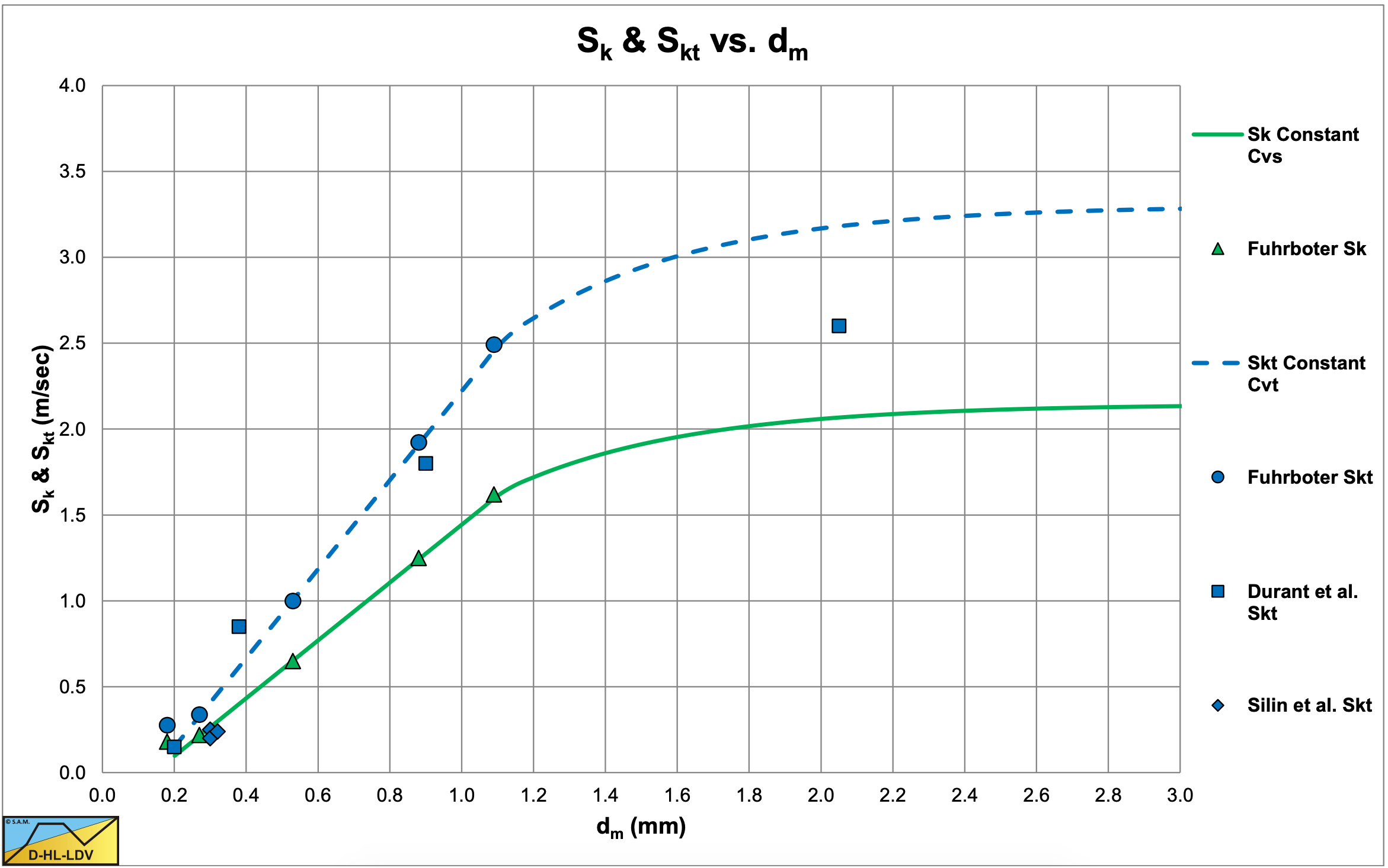
The coefficient S_kt is an emperical coefficient depending on the solids properties according to Figure 6.7-5 and equation (6.7-7) as found in many textbooks, but not in Fuhrboter (1961).

\[\ \begin{array}{ll}\mathrm{S}_{\mathrm{k t}}=\text { not defined } & \mathrm{d}_{\mathrm{m}}<\mathrm{0 . 2} \mathrm{~ m m} \\ \mathrm{S}_{\mathrm{k t}}=2 . \mathrm{5 9} \cdot \mathrm{d}_{\mathrm{m}}-\mathrm{0 . 3 7} & \mathrm{0 . 2} \mathrm{~ m m} \leq \mathrm{d}_{\mathrm{m}}<\mathrm{1 . 1} \mathrm{~ m m} \\ \mathrm{S}_{\mathrm{k t}}=\mathrm{a c c o r d i n g} \text { to graph } & \mathrm{1 . 1} \mathrm{~ m m} \leq \mathrm{d}_{\mathrm{m}}<\mathrm{3 . 0} \mathrm{~ m m} \\ \mathrm{S}_{\mathrm{k t}} \approx \mathrm{3 . 3} & \mathrm{3 . 0} \mathrm{~ m m} \leq \mathrm{d}_{\mathrm{m}}\end{array}\]

Note that the particle diameter is in mm not in m and the graph is for sand. The model of Fuhrboter is very easy to use and to calibrate with own data. The transport factor S_kt however has to cover all the effects of the frictional head loss, like the soil properties, the settling process and the liquid properties. Furthermore, the assumption of a constant slip factor is unacceptable for different soils and flow conditions. The conclusion is that the model is only applicable for the conditions in which the experiments of Fuhrboter were carried out.

Equation (6.7-6) can be written in a more general form as:

\[\ \begin{array} \Delta \mathrm{p}_{\mathrm{m}}=\Delta \mathrm{p}_{\mathrm{l}} \cdot\left(\mathrm{1}+\mathrm{2} \cdot\left(\mathrm{g} \cdot \mathrm{D}_{\mathrm{p}} \cdot \mathrm{R}_{\mathrm{s d}}\right) \cdot\left(\frac{\mathrm{S}_{\mathrm{k} \mathrm{t}}}{\lambda_{\mathrm{l}} \cdot \mathrm{R}_{\mathrm{s d}}}\right) \cdot \mathrm{C}_{\mathrm{v t}} \cdot\left(\frac{\mathrm{1}}{\mathrm{v}_{\mathrm{l s}}}\right)^{3}\right)\\
\mathrm{i}_{\mathrm{m}}=\mathrm{i}_{\mathrm{l}}+\mathrm{S}_{\mathrm{k t}} \cdot \mathrm{C}_{\mathrm{v} \mathrm{t}} \cdot \frac{\mathrm{1}}{\mathrm{v}_{\mathrm{l} \mathrm{s}}}\end{array}\]

Substituting equation (6.7-7) gives for 0.2 mm \(\ \leq\) d_m < 1.1 mm :

\[\ \Delta \mathrm{p}_{\mathrm{m}}=\Delta \mathrm{p}_{\mathrm{l}} \cdot\left(\mathrm{1}+\left(\mathrm{3 1 4 0} \cdot \mathrm{d}_{\mathrm{m}}-\mathrm{4 4 8}\right) \cdot \frac{\mathrm{g} \cdot \mathrm{D}_{\mathrm{p}} \cdot \mathrm{R}_{\mathrm{s} \mathrm{d}}}{\lambda_{\mathrm{l}}} \cdot \mathrm{C}_{\mathrm{v} \mathrm{t}} \cdot\left(\frac{\mathrm{1}}{\mathrm{v}_{\mathrm{l s}}}\right)^{3}\right)\]

With λ_l=0.015 and R_sd =1.65 this would give:

\[\ \Delta \mathrm{p}_{\mathrm{m}}=\Delta \mathrm{p}_{\mathrm{l}} \cdot\left(\mathrm{1}+\mathrm{2} \cdot\left(\mathrm{g} \cdot \mathrm{D}_{\mathrm{p}} \cdot \mathrm{R}_{\mathrm{s d}}\right) \cdot\left(\mathrm{4 0} \cdot \mathrm{S}_{\mathrm{k t}}\right) \cdot \mathrm{C}_{\mathrm{v t}} \cdot\left(\frac{\mathrm{1}}{\mathrm{v}_{\mathrm{l s}}}\right)^{\mathrm{3}}\right)\]

As stated above, the fixed slip factor of 0.65 was based on the propagation velocity of density waves. The question is whether or not this propagation velocity is a good measure for the slip factor or slip velocity. According to Matousek (1997) the propagation of density waves is a very complex process which is not directly related to the slip velocity of the solids. Yagi et al. (1972), Matousek (1996), Grunsven (2012) and others found that the slip velocity in the heterogeneous regime is just a few percent near the Limit Deposit Velocity and less than 1 percent near the homogeneous regime. In general, the slip can be neglected in the heterogeneous regime. The assumption of a slip factor of 0.65 as used by Fuhrboter (1961) is thus rejected and the conclusion is that the S_k value should be applied and not the S_kt value, giving:

\[\ \begin{array}{ll}\mathrm{S}_{\mathrm{k}}=\text { not defined } & \mathrm{d}_{\mathrm{m}}<\mathrm{0 . 2} \mathrm{~ m m} \\ \mathrm{S}_{\mathrm{k}}=\mathrm{1 . 6 8} \cdot \mathrm{d}_{\mathrm{m}}-\mathrm{0 . 2 4} & \mathrm{0 . 2} \mathrm{~ m m} \leq \mathrm{d}_{\mathrm{m}}<\mathrm{1 . 1} \mathrm{~ m m} \\ \mathrm{S}_{\mathrm{k}}=\text { according to graph } & \mathrm{1 . 1} \mathrm{~ m m} \leq \mathrm{d}_{\mathrm{m}}<\mathrm{3 . 0} \mathrm{~ m m} \\ \mathrm{S}_{\mathrm{k}} \approx 2.1 \mathrm{5} & \mathrm{3 . 0} \mathrm{~ m m} \leq \mathrm{d}_{\mathrm{m}}\end{array}\]

Equation (6.7-3) can be written in a more general form as:

\[\ \begin{array} \Delta \mathrm{p}_{\mathrm{m}}=\Delta \mathrm{p}_{\mathrm{l}} \cdot\left(\mathrm{1}+\mathrm{2} \cdot\left(\mathrm{g} \cdot \mathrm{D}_{\mathrm{p}} \cdot \mathrm{R}_{\mathrm{s} \mathrm{d}}\right) \cdot\left(\frac{\mathrm{S}_{\mathrm{k}}}{\lambda_{\mathrm{l}} \cdot \mathrm{R}_{\mathrm{s d}}}\right) \cdot \mathrm{C}_{\mathrm{v} \mathrm{s}} \cdot\left(\frac{\mathrm{1}}{\mathrm{v}_{\mathrm{ls}}}\right)^{3}\right)\\
\mathrm{i}_{\mathrm{m}}=\mathrm{i}_{\mathrm{l}}+\mathrm{S}_{\mathrm{k}} \cdot \mathrm{C}_{\mathrm{v} \mathrm{s}} \cdot \frac{\mathrm{l}}{\mathrm{v}_{\mathrm{ls}}}\end{array}\]

Substituting equation (6.7-11) gives for 0.2 mm \(\ \leq\) d_m < 1.1 mm :

\[\ \Delta \mathrm{p}_{\mathrm{m}}=\Delta \mathrm{p}_{\mathrm{l}} \cdot\left(\mathrm{1}+\left(\mathrm{2 0 4 1} \cdot \mathrm{d}_{\mathrm{m}}-\mathrm{2 9 1}\right) \cdot \frac{\mathrm{g} \cdot \mathrm{D}_{\mathrm{p}} \cdot \mathrm{R}_{\mathrm{s d}}}{\lambda_{\mathrm{l}}} \cdot \mathrm{C}_{\mathrm{v s}} \cdot\left(\frac{\mathrm{1}}{\mathrm{v}_{\mathrm{l s}}}\right)^{3}\right)\]

With λ_l=0.015 and R_sd =1.65 this would give:

\[\ \Delta \mathrm{p}_{\mathrm{m}}=\Delta \mathrm{p}_{\mathrm{l}} \cdot\left(\mathrm{1}+\mathrm{2} \cdot\left(\mathrm{g} \cdot \mathrm{D}_{\mathrm{p}} \cdot \mathrm{R}_{\mathrm{s d}}\right) \cdot\left(\mathrm{4 0} \cdot \mathrm{S}_{\mathrm{k}}\right) \cdot \mathrm{C}_{\mathrm{v s}} \cdot\left(\frac{\mathrm{1}}{\mathrm{v}_{\mathrm{l s}}}\right)^{3}\right)\]

It should be mentioned that Fuhrboter (1961) found excess pressure losses that decreased with the line speed, but with a power a bit higher than -1 in equation (6.7-3), like -1.2, which would result in a power of about 3.2 in the above equations. This matches the findings of Wilson et al. (1992), who found a power of -1.7 for uniform sands, decreasing to -0.25 for very graded sands. Fuhrboter (1961) also used the mean particle diameter d_m instead of the d₅₀. Although there are small differences for the sands used, this will not lead to a significant change in the S_k graph, so the graph can also be used with the d₅₀.

Figure 6.7-6 shows that the DHLLDV Framework for graded sands may explain the steepness of the data points, which is less steep than for uniform sands.

Finally Figure 6.7-7 shows a lower and upper limit to the S_k value based on the DHLLDV Framework at 20^oC. At other temperatures the curves may be slightly different. A lower temperature gives higher curves.

Figure 6.7-6: The data of Fuhrboter with a d₅₀=0.83 mm sand compared with the DHLLDV Framework for a graded sand.

Figure 6.7-7: S_k lower and upper limit based on the DHLLDV Framework.