6.20: Charles (1970) and Babcock (1970)
- Page ID
- 30849

\( \newcommand{\vecs}[1]{\overset { \scriptstyle \rightharpoonup} {\mathbf{#1}} } \)
\( \newcommand{\vecd}[1]{\overset{-\!-\!\rightharpoonup}{\vphantom{a}\smash {#1}}} \)
\( \newcommand{\id}{\mathrm{id}}\) \( \newcommand{\Span}{\mathrm{span}}\)
( \newcommand{\kernel}{\mathrm{null}\,}\) \( \newcommand{\range}{\mathrm{range}\,}\)
\( \newcommand{\RealPart}{\mathrm{Re}}\) \( \newcommand{\ImaginaryPart}{\mathrm{Im}}\)
\( \newcommand{\Argument}{\mathrm{Arg}}\) \( \newcommand{\norm}[1]{\| #1 \|}\)
\( \newcommand{\inner}[2]{\langle #1, #2 \rangle}\)
\( \newcommand{\Span}{\mathrm{span}}\)
\( \newcommand{\id}{\mathrm{id}}\)
\( \newcommand{\Span}{\mathrm{span}}\)
\( \newcommand{\kernel}{\mathrm{null}\,}\)
\( \newcommand{\range}{\mathrm{range}\,}\)
\( \newcommand{\RealPart}{\mathrm{Re}}\)
\( \newcommand{\ImaginaryPart}{\mathrm{Im}}\)
\( \newcommand{\Argument}{\mathrm{Arg}}\)
\( \newcommand{\norm}[1]{\| #1 \|}\)
\( \newcommand{\inner}[2]{\langle #1, #2 \rangle}\)
\( \newcommand{\Span}{\mathrm{span}}\) \( \newcommand{\AA}{\unicode[.8,0]{x212B}}\)
\( \newcommand{\vectorA}[1]{\vec{#1}} % arrow\)
\( \newcommand{\vectorAt}[1]{\vec{\text{#1}}} % arrow\)
\( \newcommand{\vectorB}[1]{\overset { \scriptstyle \rightharpoonup} {\mathbf{#1}} } \)
\( \newcommand{\vectorC}[1]{\textbf{#1}} \)
\( \newcommand{\vectorD}[1]{\overrightarrow{#1}} \)
\( \newcommand{\vectorDt}[1]{\overrightarrow{\text{#1}}} \)
\( \newcommand{\vectE}[1]{\overset{-\!-\!\rightharpoonup}{\vphantom{a}\smash{\mathbf {#1}}}} \)
\( \newcommand{\vecs}[1]{\overset { \scriptstyle \rightharpoonup} {\mathbf{#1}} } \)
\( \newcommand{\vecd}[1]{\overset{-\!-\!\rightharpoonup}{\vphantom{a}\smash {#1}}} \)
\(\newcommand{\avec}{\mathbf a}\) \(\newcommand{\bvec}{\mathbf b}\) \(\newcommand{\cvec}{\mathbf c}\) \(\newcommand{\dvec}{\mathbf d}\) \(\newcommand{\dtil}{\widetilde{\mathbf d}}\) \(\newcommand{\evec}{\mathbf e}\) \(\newcommand{\fvec}{\mathbf f}\) \(\newcommand{\nvec}{\mathbf n}\) \(\newcommand{\pvec}{\mathbf p}\) \(\newcommand{\qvec}{\mathbf q}\) \(\newcommand{\svec}{\mathbf s}\) \(\newcommand{\tvec}{\mathbf t}\) \(\newcommand{\uvec}{\mathbf u}\) \(\newcommand{\vvec}{\mathbf v}\) \(\newcommand{\wvec}{\mathbf w}\) \(\newcommand{\xvec}{\mathbf x}\) \(\newcommand{\yvec}{\mathbf y}\) \(\newcommand{\zvec}{\mathbf z}\) \(\newcommand{\rvec}{\mathbf r}\) \(\newcommand{\mvec}{\mathbf m}\) \(\newcommand{\zerovec}{\mathbf 0}\) \(\newcommand{\onevec}{\mathbf 1}\) \(\newcommand{\real}{\mathbb R}\) \(\newcommand{\twovec}[2]{\left[\begin{array}{r}#1 \\ #2 \end{array}\right]}\) \(\newcommand{\ctwovec}[2]{\left[\begin{array}{c}#1 \\ #2 \end{array}\right]}\) \(\newcommand{\threevec}[3]{\left[\begin{array}{r}#1 \\ #2 \\ #3 \end{array}\right]}\) \(\newcommand{\cthreevec}[3]{\left[\begin{array}{c}#1 \\ #2 \\ #3 \end{array}\right]}\) \(\newcommand{\fourvec}[4]{\left[\begin{array}{r}#1 \\ #2 \\ #3 \\ #4 \end{array}\right]}\) \(\newcommand{\cfourvec}[4]{\left[\begin{array}{c}#1 \\ #2 \\ #3 \\ #4 \end{array}\right]}\) \(\newcommand{\fivevec}[5]{\left[\begin{array}{r}#1 \\ #2 \\ #3 \\ #4 \\ #5 \\ \end{array}\right]}\) \(\newcommand{\cfivevec}[5]{\left[\begin{array}{c}#1 \\ #2 \\ #3 \\ #4 \\ #5 \\ \end{array}\right]}\) \(\newcommand{\mattwo}[4]{\left[\begin{array}{rr}#1 \amp #2 \\ #3 \amp #4 \\ \end{array}\right]}\) \(\newcommand{\laspan}[1]{\text{Span}\{#1\}}\) \(\newcommand{\bcal}{\cal B}\) \(\newcommand{\ccal}{\cal C}\) \(\newcommand{\scal}{\cal S}\) \(\newcommand{\wcal}{\cal W}\) \(\newcommand{\ecal}{\cal E}\) \(\newcommand{\coords}[2]{\left\{#1\right\}_{#2}}\) \(\newcommand{\gray}[1]{\color{gray}{#1}}\) \(\newcommand{\lgray}[1]{\color{lightgray}{#1}}\) \(\newcommand{\rank}{\operatorname{rank}}\) \(\newcommand{\row}{\text{Row}}\) \(\newcommand{\col}{\text{Col}}\) \(\renewcommand{\row}{\text{Row}}\) \(\newcommand{\nul}{\text{Nul}}\) \(\newcommand{\var}{\text{Var}}\) \(\newcommand{\corr}{\text{corr}}\) \(\newcommand{\len}[1]{\left|#1\right|}\) \(\newcommand{\bbar}{\overline{\bvec}}\) \(\newcommand{\bhat}{\widehat{\bvec}}\) \(\newcommand{\bperp}{\bvec^\perp}\) \(\newcommand{\xhat}{\widehat{\xvec}}\) \(\newcommand{\vhat}{\widehat{\vvec}}\) \(\newcommand{\uhat}{\widehat{\uvec}}\) \(\newcommand{\what}{\widehat{\wvec}}\) \(\newcommand{\Sighat}{\widehat{\Sigma}}\) \(\newcommand{\lt}{<}\) \(\newcommand{\gt}{>}\) \(\newcommand{\amp}{&}\) \(\definecolor{fillinmathshade}{gray}{0.9}\)6.9.1 Charles (1970)
The models of Durand & Condolios (1952), Newitt et al. (1955), Worster & Denny (1955), Fuhrboter (1961), Jufin & Lopatin (1966) and Zandi & Govatos (1967) all have in common that the equation for the excess head losses in the heterogeneous regime approaches zero for very high line speeds. Charles (1970) states that this cannot be true, since in general the excess head losses will approach the excess head losses matching the ELM. In other words, for very high line speeds the hydraulic gradient should be determined with the Darcy Weisbach equation, replacing the density of the pure liquid with the mixture density. Most equations have the following form, or can be rewritten to this form:
\[\ \Phi=\frac{\mathrm{i}_{\mathrm{m}}-\mathrm{i}_{\mathrm{l}}}{\mathrm{i}_{\mathrm{l}} \cdot \mathrm{C}_{\mathrm{v t}}}=\mathrm{K} \cdot \Psi^{-\beta}\]
With:
\[\ \Psi=\left(\frac{\mathrm{v}_{\mathrm{l} \mathrm{s}}^{2}}{\mathrm{g} \cdot \mathrm{D}_{\mathrm{p}} \cdot \mathrm{R}_{\mathrm{s d}}}\right) \cdot \sqrt{\mathrm{C}_{\mathrm{x}}} \quad\text{ or }\quad \Psi=\left(\frac{\mathrm{v}_{\mathrm{l} s}^{2}}{\mathrm{g} \cdot \mathrm{D}_{\mathrm{p}} \cdot \mathrm{R}_{\mathrm{s d}}}\right) \cdot \sqrt{\mathrm{C}_{\mathrm{D}}}\]
Durand & Condolios (1952) use the first variant, while both Charles (1970) and Babcock (1970) use the second variant. The difference between the two variants is significant and should be taken into account when using this equation. For the factor K values in the range of 80-150 have been found. The original Durand & Condolios (1952) equation did not mention a value, however later values in the range of 80-85 are deduced. The value of β=1.5 for the heterogeneous regime, although values up to 2 are found in literature. In order to get a smooth transition from the heterogeneous regime to the homogeneous regime, Charles (1970) suggested the following equation:
\[\ \Phi=\frac{\mathrm{i}_{\mathrm{m}}-\mathrm{i}_{\mathrm{l}}}{\mathrm{i}_{\mathrm{l}} \cdot \mathrm{C}_{\mathrm{v t}}}=\mathrm{K} \cdot \Psi^{-\beta}+\mathrm{R}_{\mathrm{s d}}\]
Or for the relative excess hydraulic gradient:
\[\ \mathrm{E}_{\mathrm{rhg}}=\frac{\mathrm{i}_{\mathrm{m}}-\mathrm{i}_{\mathrm{l}}}{\mathrm{C}_{\mathrm{v}} \cdot \mathrm{R}_{\mathrm{sd}}}=\mathrm{i}_{\mathrm{l}} \cdot\left(\frac{\mathrm{K}}{\mathrm{R}_{\mathrm{sd}}} \cdot \Psi^{-\beta}+1\right)\]
The disadvantage of this equation is, that the hydraulic gradient can never be smaller than the ELM, which is often observed to be the case. However as an upper limit to the hydraulic gradient the equation is useful. Charles (1970) also suggested to use the Minimum Hydraulic Gradient Velocity (MHGV) as an estimate for the Limit Deposit Velocity (LDV) since these are close. This MHGV can be obtained by differentiating the above equation with respect to the line speed vls. This gives:
\[\ \mathrm{i}_{\mathrm{m}}=\mathrm{i}_{\mathrm{l}} \cdot\left(\frac{\mathrm{K}}{\mathrm{R}_{\mathrm{s d}}} \cdot \Psi^{-\beta}+\mathrm{1}\right) \cdot \mathrm{C}_{\mathrm{v} \mathrm{t}} \cdot \mathrm{R}_{\mathrm{sd}}+\mathrm{i}_{\mathrm{l}}\]
Or:
\[\ \begin{aligned} \mathrm{i}_{\mathrm{m}} =\frac{\lambda_{\mathrm{l}} \cdot \mathrm{v}_{\mathrm{l} \mathrm{s}}^{2}}{\mathrm{2} \cdot \mathrm{g} \cdot \mathrm{D}_{\mathrm{p}}} \cdot\left(\frac{\mathrm{K}}{\mathrm{R}_{\mathrm{s} \mathrm{d}}} \cdot\left(\left(\frac{\mathrm{v}_{\mathrm{l} \mathrm{s}}^{2}}{\mathrm{g} \cdot \mathrm{D}_{\mathrm{p}} \cdot \mathrm{R}_{\mathrm{s d}}}\right) \cdot \sqrt{\mathrm{C}_{\mathrm{x}}}\right)^{-\mathrm{1 . 5}}+\mathrm{1}\right) \cdot \mathrm{C}_{\mathrm{v} \mathrm{t}} \cdot \mathrm{R}_{\mathrm{s d}}+\frac{\lambda_{\mathrm{l}} \cdot \mathrm{v}_{\mathrm{l} \mathrm{s}}^{2}}{\mathrm{2} \cdot \mathrm{g} \cdot \mathrm{D}_{\mathrm{p}}}\\
\left.\mathrm{i}_{\mathrm{m}} =\frac{\lambda_{\mathrm{l}}}{\mathrm{2} \cdot \mathrm{g} \cdot \mathrm{D}_{\mathrm{p}}} \cdot\left(\mathrm{1}+\mathrm{C}_{\mathrm{v} \mathrm{t}} \cdot \mathrm{R}_{\mathrm{s d}}\right) \cdot \mathrm{v}_{\mathrm{l} \mathrm{s}}^{2}+\left(\mathrm{K} \cdot\left(\frac{\mathrm{g} \cdot \mathrm{D}_{\mathrm{p}} \cdot \mathrm{R}_{\mathrm{s d}}}{\sqrt{\mathrm{C}_{\mathrm{x}}}}\right)^{1.5} \cdot \mathrm{C}_{\mathrm{v} \mathrm{t}}\right) \cdot \frac{\mathrm{1}}{\mathrm{v}_{\mathrm{l s}}}\right)\end{aligned}\]
This gives for the MHGV:
\[\ \mathrm{v}_{\mathrm{l s}, \mathrm{M H G V}}=\left(\frac{\left.(\mathrm{K} \cdot\left(\frac{\mathrm{g} \cdot \mathrm{D}_{\mathrm{p}} \cdot \mathrm{R}_{\mathrm{s d}}}{\sqrt{\mathrm{C}_{\mathrm{x}}}}\right)^{1.5} \cdot \mathrm{C}_{\mathrm{v t}}\right)}{\mathrm{2} \cdot\left(\mathrm{1}+\mathrm{C}_{\mathrm{v t}} \cdot \mathrm{R}_{\mathrm{s d}}\right)}\right)^{1 / 3}\]
6.9.2 Babcock (1970)
Babcock (1970) adopted the approach of Charles (1970) regarding the transition of the heterogeneous regime to the homogeneous regime. The disadvantage of adding two possible solutions without any correction will probably overestimate the hydraulic gradient near the intersection point of the two regimes. The Wasp et al. (1977) model by means of the vehicle concentration and the Wilson et al (2006) model by means of the stratification ratio, do take this into account.
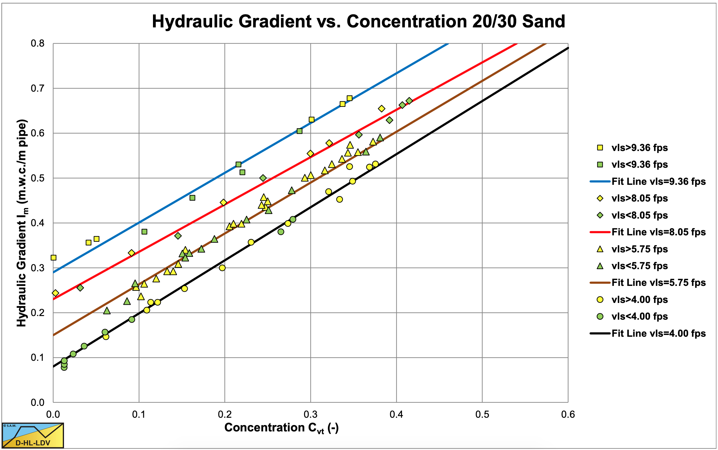
The excess hydraulic gradient, the difference between the mixture hydraulic gradient and the pure liquid hydraulic gradient, is supposed to be proportional to the concentration of solids by volume in the mixture, the proportionality assumption. Now it is not always clear what is meant by the concentration of solids by volume in the mixture. The definition points to the spatial concentration, however most researchers have used the delivered concentration. A second assumption as used by Babcock (1970) is adopted from Durand & Condolios (1952), the size independence assumption for coarse particles. Stating that the excess hydraulic gradient is independent of the particle size above a certain particle diameter. The purpose of the research of Babcock (1970) was to verify these assumptions. The research was carried out in a 0.0254 m diameter pipe (1 inch). The first experiments were carried out with a 20/30 mesh quartz sand (coarse). The results are shown in Figure 6.9-1 and show a linear relation between the hydraulic gradient and the volumetric concentration. The equation of these lines is, using equation (6.9-2):
\[\ \Phi=\frac{\mathrm{i}_{\mathrm{m}}-\mathrm{i}_{\mathrm{l}}}{\mathrm{i}_{\mathrm{l}} \cdot \mathrm{C}_{\mathrm{v t}}}=7 \mathrm{0} \cdot \Psi^{-1}\]
Inspection of the flow revealed that all of these experiments were in the sliding bed regime. The above equation is very similar to the Newitt et al. (1955) equation.
Next a series of tests were carried out with an 80/100 mesh quartz sand (fine). The results of these experiments are shown in Figure 6.9-2. Up to a volumetric concentration of 20-25% the relation is linear, but above 25% the excess hydraulic gradient starts increasing more than linear. Inspection of the flow showed that at low concentrations most of the material was travelling as suspended load, but at higher concentrations there was a sliding bed and at the highest concentrations even a stationary bed. The following equation was derived from the experiments:
\[\ \Phi=\frac{\mathrm{i}_{\mathrm{m}}-\mathrm{i}_{\mathrm{l}}}{\mathrm{i}_{\mathrm{l}} \cdot \mathrm{C}_{\mathrm{v t}}}=\mathrm{6 . 3} \cdot \Psi^{-\mathrm{0 . 2 5 4}}\]
Note that this equation is very similar to the Zandi & Govatos (1967) equation for pseudo homogeneous flow. The equation correlates well for concentrations up to 20%.
At last a series of experiments were conducted with a 30/45 mesh quartz sand (medium). The results are shown in Figure 6.9-3. Now it seems there is a curvature between 10% and 25% volumetric concentration, while the line straightens for the higher concentrations.
Similar tests were run on 6/8 mesh steel shot, on 10/16 mesh arkosic sand and on 16/30 mesh garnet sand. The results of these experiments are shown in Figure 6.9-4 and Figure 6.9-5, showing the same data points but with a different abscissa and ordinate. These tests clearly showed the occurrence of a sliding bed. The equation following from these experiments is:
\[\ \frac{\mathrm{i}_{\mathrm{m}}-\mathrm{i}_{\mathrm{l}}}{\mathrm{i}_{\mathrm{l}} \cdot \mathrm{C}_{\mathrm{v t}} \cdot \mathrm{R}_{\mathrm{s d}}}=\mathrm{6 0 . 6} \cdot\left(\frac{\mathrm{v}_{\mathrm{l} \mathrm{s}}^{2}}{\mathrm{g} \cdot \mathrm{D}_{\mathrm{p}}}\right)^{-\mathrm{1}}\text{
or }\quad \Phi=\frac{\mathrm{i}_{\mathrm{m}}-\mathrm{i}_{\mathrm{l}}}{\mathrm{i}_{\mathrm{l}} \cdot \mathrm{C}_{\mathrm{v t}}}=60.6 \cdot\left(\frac{\mathrm{v}_{\mathrm{l} s}^{2}}{\mathrm{g} \cdot \mathrm{R}_{\mathrm{s d}} \cdot \mathrm{D}_{\mathrm{p}}}\right)^{-1}=\mathrm{6 0 . 6 \cdot \Psi}^{-\mathrm{1}}\]
The above equation is very similar to the Newitt et al. (1955) equation. Newitt et al. (1955) found a factor of 66, Babcock (1970) a factor of 70 and a factor of 60.6. These values are very close. With a normal Darcy Weisbach friction factor of about 0.020-0.025 for a 0.0254 m diameter pipe this gives a sliding friction factor of μsf=0.6- 0.875. This is comparable to Newitt et al. (1955).
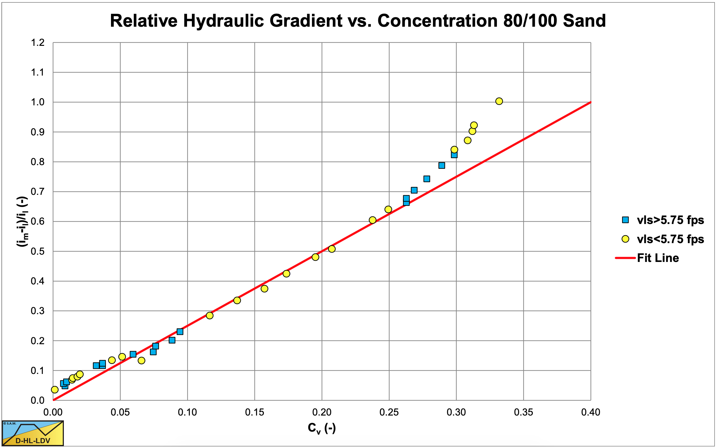
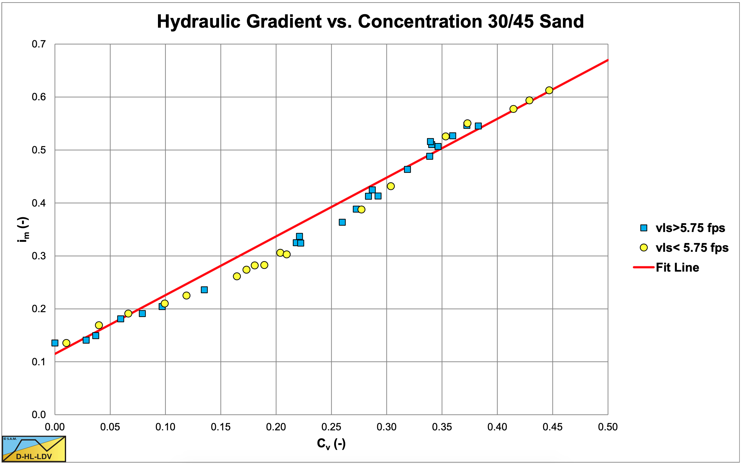
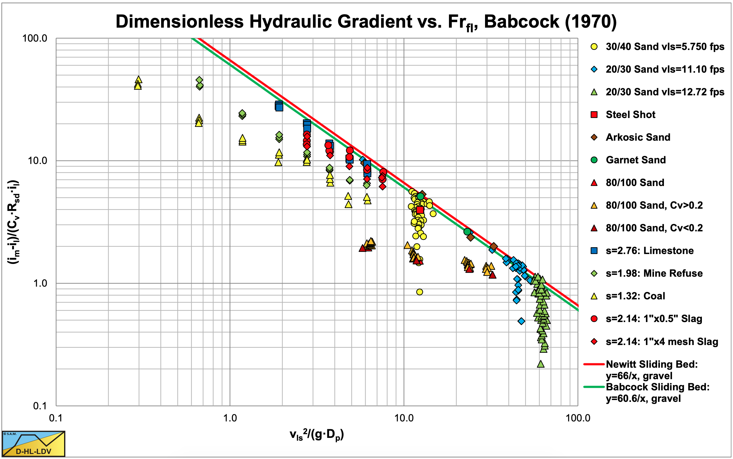
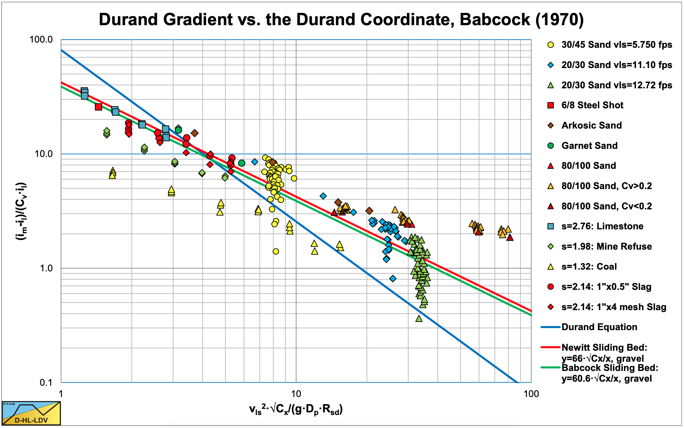
Figure 6.9-4 uses the original abscissa and ordinate, Figure 6.9-5 the abscissa and ordinate according to Durand & Condolios (1952).
It is not always clear whether the spatial or the delivered volumetric concentration is used, but for high line speeds there is not much difference.
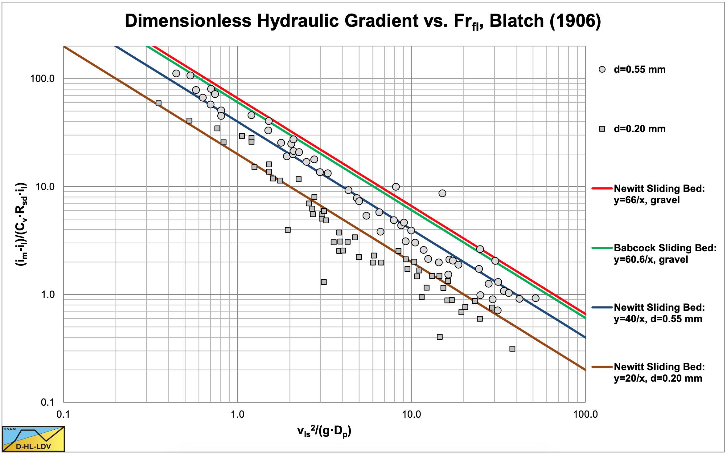
Babcock (1970) also compared the experimental data of Nora Stanton Blatch (1906) in similar graphs. The first experiments discovered were carried out by Nora Stanton Blatch (1906), with a pipeline of 1 inch and sand particles of d=0.15-0.25 mm and d=0.4-0.8 mm. At high line speeds, the solids effect is decreasing. Figure 6.9-9 and Figure 6.9-8 show the data points, normalized to a volumetric concentration of 20%.
The data points of Blatch show a considerable scatter, but if one considers the experiments were carried out in 1906, the data points do point in a certain direction. Since the real concentrations are not known, all data points are normalized to a concentration of 10%. In general, the data points follow the sliding bed curves.
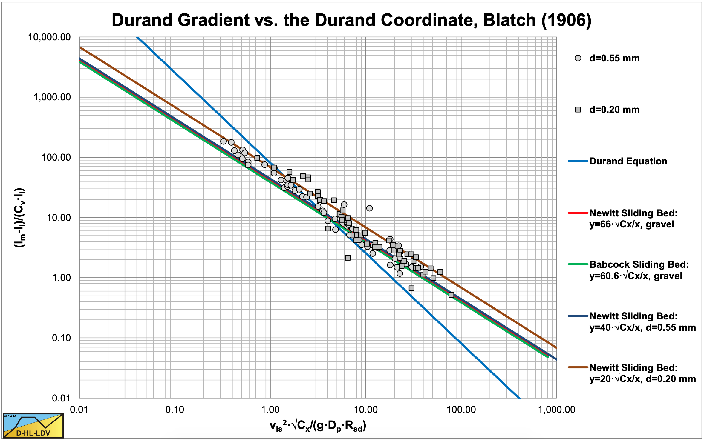
Figure 6.9-6 shows the data points in a different coordinate system. For the transformation to Durand coordinates, a relative submerged density of Rsd =1.65 and a particle Froude number of Fr-1=√Cx=1.2/3.42 are assumed. The tests were carried out in a 1 inch pipe with d=0.20 mm and d=0.55 mm sand. The Fr-1=√Cx is determined with the Gibert (1960) graph. The data points seem to be parallel to the Newitt et al. (1955) and Babcock sliding bed curves, while the steepness looks a bit smaller than the Durand curve. This could point to a sliding bed and/or sheet flow. Nora Stanton Blatch (1906) however did not give a theoretical explanation of the phenomena she observed.
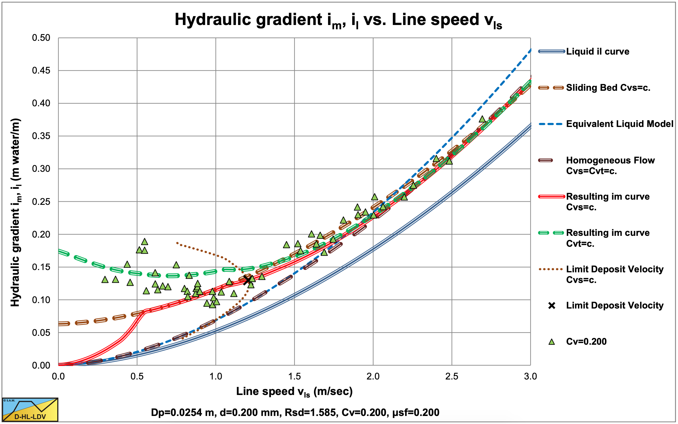
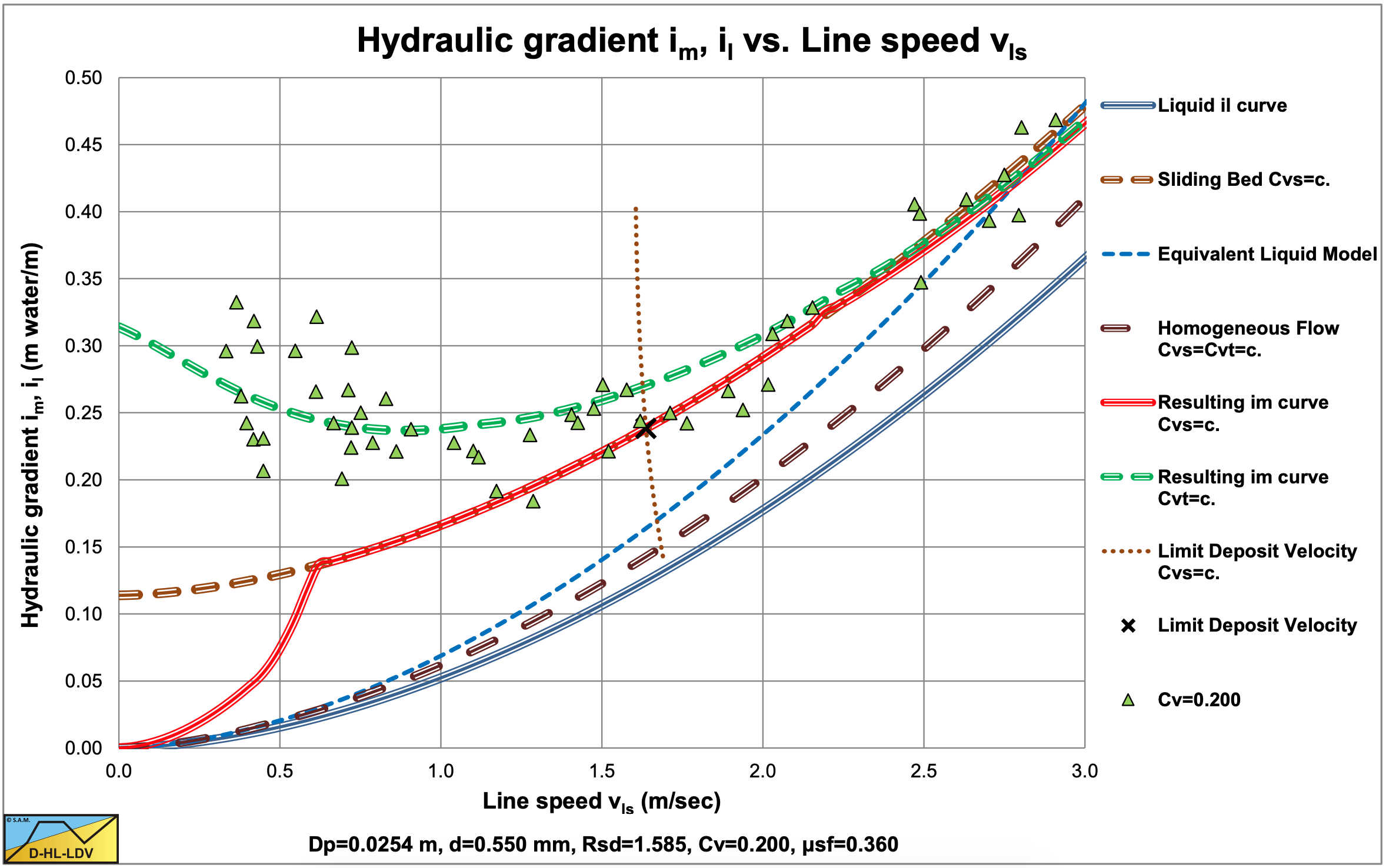
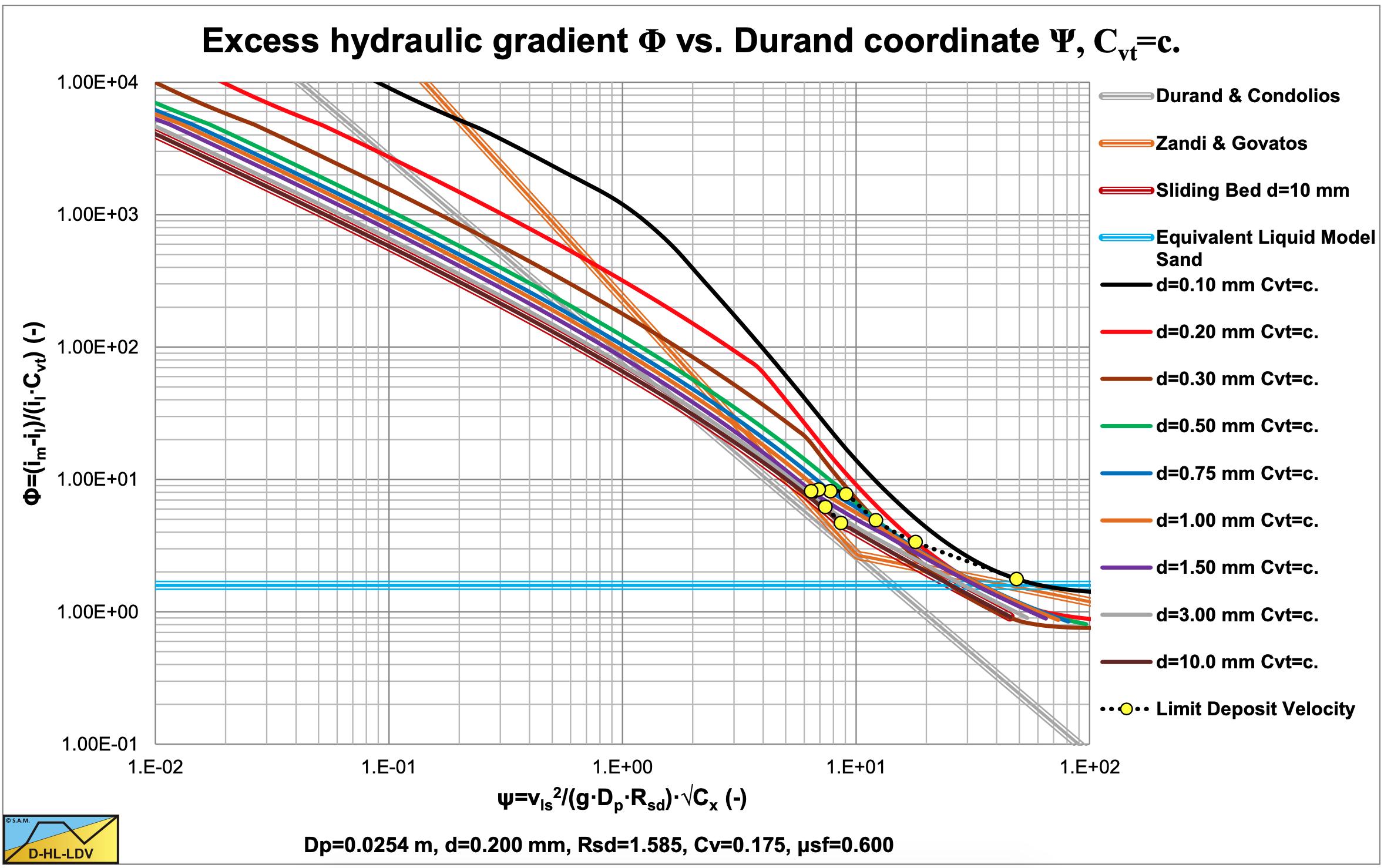
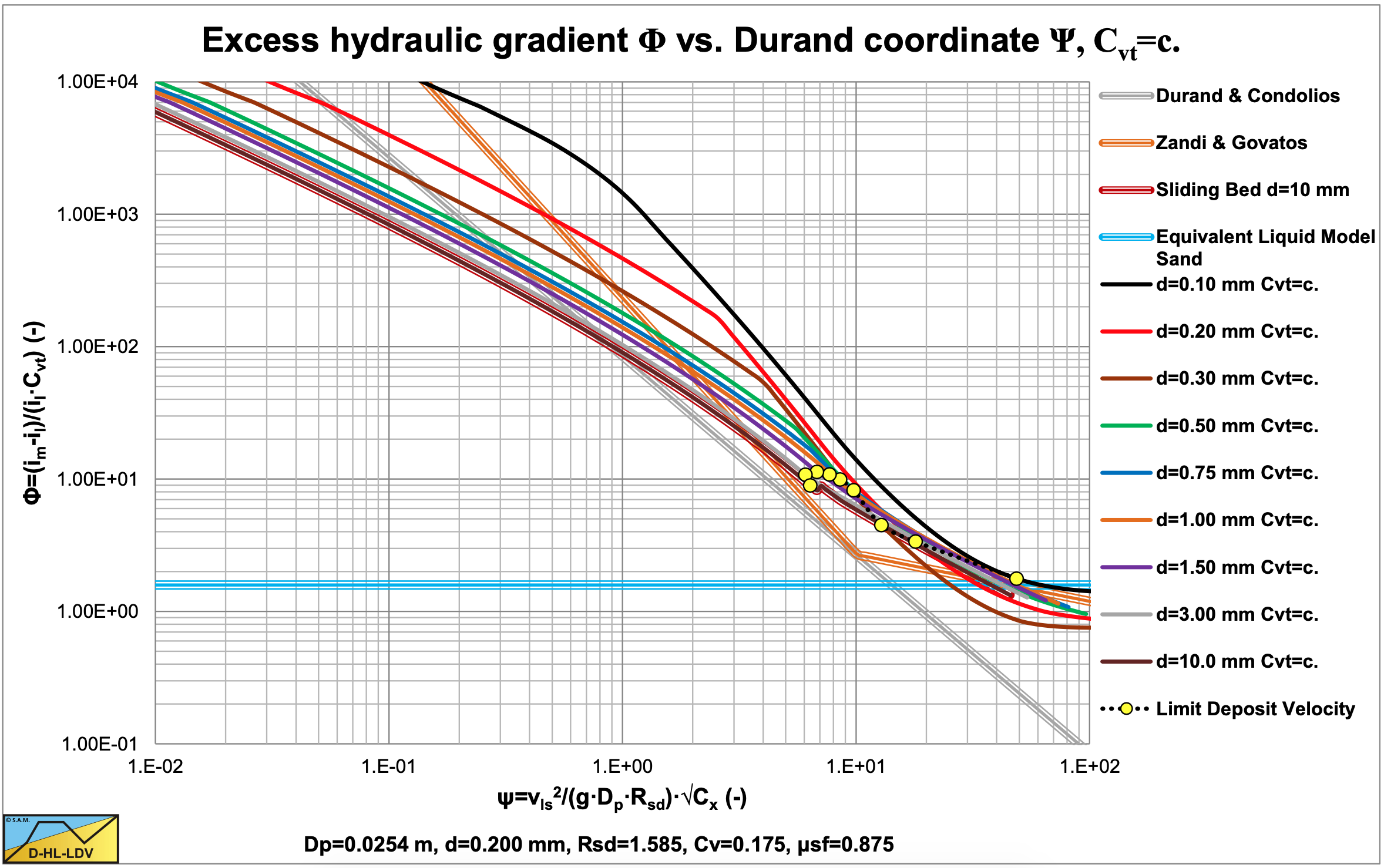
Figure 6.9-10 and Figure 6.9-11 show the results of the DHLLDV Framework for the range of parameters as used by Babcock (1970). These simulations match the data of Babcock (1970) very well.
The most important observations of Babcock (1970) however are the confirmation of the proportionality of the excess head losses with the volumetric concentration. Although at high concentrations fine particles show some non-linear behavior, for medium and coarse particles in the sliding bed regime the proportionality has been proven. These findings contradict the hydrostatic normal stress approach of Wilson et al. (2006), which would have shown a more than linear increase of the excess head losses with increasing volumetric concentration. These findings confirm the weight approach of Miedema & Ramsdell (2014) assuming a linear relation.