6.23: The Kaushal and Tomita (2002B) Model

6.23.1 Introduction

Kaushal with changing co-authors developed a model for predicting the hydraulic gradient in horizontal pipelines, based on a modified Wasp et al. (1977) model and a modified Karabelas (1977) model. First the different papers are discussed in the right chronological order, after which the model is discussed in detail.

Kaushal et al. (2002A) describe the concentration distribution and the concentration at the pipe bottom at the deposition velocity. The concentration distribution is based on the advection diffusion equation as originally presented by O’Brien (1933) and Rouse (1937) and modified for the upwards flow of the liquid at higher concentrations by Hunt (1954). The original advection diffusion equation gives:

\[\ \mathrm{v}_{\mathrm{t}} \cdot \mathrm{C}_{\mathrm{v s}}(\mathrm{z})+\varepsilon_{\mathrm{s}} \cdot \frac{\partial \mathrm{C}_{\mathrm{v s}}(\mathrm{z})}{\partial \mathrm{z}}=0\]

The advection diffusion equation as modified by Hunt (1954) gives:

\[\ \mathrm{v}_{\mathrm{t}} \cdot \mathrm{C}_{\mathrm{v} \mathrm{s}}(\mathrm{z}) \cdot\left(1-\mathrm{C}_{\mathrm{v s}}(\mathrm{z})\right)+\varepsilon_{\mathrm{s}} \cdot \frac{\partial \mathrm{C}_{\mathrm{v s}}(\mathrm{z})}{\partial \mathrm{z}}=0\]

Giving, in case of constant diffusivity and no hindered settling for uniform sands:

\[\ \mathrm{C_{v s}(z)=\frac{\frac{C_{v B}}{1-C_{v B}} \cdot e^{-\frac{v_{t}}{\varepsilon_{s}} \cdot \frac{z}{D_{p}}}}{1+\frac{C_{v B}}{1-C_{v B}} \cdot e^{-\frac{v_{t}}{\varepsilon_{s}} \cdot \frac{z}{D_{p}}}}=\frac{e^{-\frac{v_{t}}{\varepsilon_{s}} \cdot \frac{z}{D_{p}}}}{\frac{1-C_{v B}}{C_{v B}}+e^{-\frac{v_{t}}{\varepsilon_{s}} \cdot \frac{z}{D_{p}}}}}\]

At the bottom of the pipe, z=0, this gives C_vs(0)=C_vB, the concentration at the bottom.

The Karabelas (1977) approach for determining the concentration distributions of graded solids is applied with some modifications. The Longwell (1977) approach for the liquid eddy momentum diffusivity is applied instead of a constant diffusivity, making the liquid eddy momentum diffusivity depending on the vertical position in the pipe. Based on Mukhtar (1991) and Kaushal (1995) the factor between the sediment diffusivity and the liquid eddy momentum diffusivity has been modified, by making it dependent on the volumetric concentration, and hindered settling has been added according to Richardson & Zaki (1954).

The new model is compared with experimental data of zinc tailings in a 0.105 m horizontal pipe, with volumetric concentrations of 3.8% to 26% and line speeds of 2 m/s to 3.5 m/s. At very low concentrations the Karabelas (1977) model and the Kaushal et al. (2002A) model give about the same results. At higher concentrations however, the Karabelas (1977) model differs from the experimental data, the higher the concentration, the bigger the difference. The Kaushal et al. (2002A) model gives a very good correlation with the experimental data.

Kaushal & Tomita (2002B) describe the Wasp et al. (1977) and the Gillies et al. (1991) methods for determining hydraulic gradients in slurry flow. The Gillies et al. (1991) method is further referred to as the SRC method and is already described in chapter 6. The Kaushal et al. (2002A) model for determining the concentration profile, the modified Karabelas (1977) model, is applied in order to find the so called Wasp et al. (1977) criterion to determine the solids fraction in suspension. In the Wasp et al. (1977) model, the calculation of the Darcy Weisbach friction factor is determined with the modified Wood (1966) equation and the factor relating the sediment diffusivity to the liquid eddy momentum diffusivity is not 1, but the equation of Kaushal et al. (2002A) is applied.

A comparison between the SRC model, the Wasp et al. (1977) model and the Kaushal & Tomita (2002B) model shows a good agreement for zinc tailings in a 0.105 m pipe at different volumetric concentrations and line speeds. At higher concentrations, up to 26%, the Wasp et al. (1977) model overestimates the experimental data, the Kaushal & Tomita (2002B) modified Wasp et al. (1977) model underestimates slightly, while the Gillies et al. (1991) model overestimates slightly.

Kaushal & Tomita (2002C) used their head loss model based on a modified Wasp et al. (1977) model, but they changed the way the suspended (vehicle) fraction is determined, based on their modified Karabelas (1977) model and not on the modified Wasp et al. (1977) equation. The factor relating the sediment diffusivity to the liquid eddy momentum diffusivity was modified compared to Kaushal et al. (2002A), including the ratio of the particle diameter of a fraction to the weighted mean diameter of the solids. The modified model was compared to the SRC model, the Wasp et al. (1977) model and the Kaushal & Tomita (2002B) model using the experimental data of the zinc tailings in a 0.105 m pipe as they used before. The Wasp et al. (1977) model overestimates the experimental data except for low line speeds, close to the LDV. The SCR model overestimates the data slightly except for low line speeds, close to the LDV. The Kaushal & Tomita (2002B) model underestimates the data for low line speeds, close to the LDV, while the Kaushal & Tomita (2002C) model gives a good match over the full range of line speeds.

Kaushal et al. (2002D) make the model applicable for rectangular ducts. The concept of the model is the same as the Kaushal & Tomita (2002C) model, but the equations for the liquid eddy momentum diffusivity and the factor relating the sediment diffusivity to the liquid eddy momentum diffusivity have been adapted to fit rectangular ducts. The model is compared with data collected by Kaushal (1995) and gives a good correlation for the concentration profiles found for different volumetric concentrations and different line speeds. Kaushal et al. (2003A) show more experimental data of experiments in a rectangular duct of 0.2 m width and 0.05 m height. Again a good correlation was found between the experiments and the model developed. Seshadri et al. (2006) also add equations for the liquid eddy momentum diffusivity.

Kaushal & Tomita (2013) improved their model with a more sophisticated factor for the relation between the sediment diffusivity and the liquid eddy momentum diffusivity, including the influence of mean particle diameter d_m to pipe diameter ratio and the influence of the grading of the PSD. This improvement resulted in a better agreement for both narrow and broad graded PSD’s.

6.23.2 The Hydraulic Gradient

The method to determine the hydraulic gradient is based on the assumption that the total hydraulic gradient in 2 phase flow can be split into two parts, the vehicle hydraulic gradient (homogeneously distributed particles) and the excess hydraulic gradient due to bed formation (heterogeneously distributed particles). An iterative method is suggested. In the prediction step the 2 phase flow is assumed to be completely homogeneous. Based on this assumption the hydraulic gradient is computed using the Darcy Weisbach equation:

\[\ \mathrm{i}_{\text {vehicle }}=\lambda_{\mathrm{m}} \cdot \frac{\mathrm{v}_{\mathrm{l s}}^{2}}{\mathrm{2} \cdot \mathrm{g} \cdot \mathrm{D}_{\mathrm{p}}} \quad\text{ or }\quad \mathrm{i}_{\text {vehicle }}=\mathrm{2} \cdot \mathrm{f}_{\mathrm{m}} \cdot \frac{\mathrm{v}_{\mathrm{l} \mathrm{s}}^{\mathrm{2}}}{\mathrm{g} \cdot \mathrm{D}_{\mathrm{p}}} \quad\text{ with: }\quad \lambda_{\mathrm{m}}=\mathrm{4} \cdot \mathrm{f}_{\mathrm{m}}\]

Kaushal & Tomita (2002B) use the Fanning friction factor f_m instead of the Darcy Weisbach friction factor λ_m.

The Fanning friction factor has been evaluated using the Wood (1966) equation in the Wasp et al. (1977) model:

\[\ \begin{array}{left}\mathrm{f}_{\mathrm{m}}=\left(\mathrm{a}+\mathrm{b} \cdot \mathrm{R} \mathrm{e}_{\mathrm{m}}^{-\mathrm{c}}\right)\\
\mathrm{a}=\mathrm{0 . 0 2 6} \cdot\left(\frac{\varepsilon}{\mathrm{D}_{\mathrm{p}}}\right)^{0.225}+\mathrm{0 . 1 3 3} \cdot\left(\frac{\varepsilon}{\mathrm{D}_{\mathrm{p}}}\right), \quad \mathrm{b}=\mathrm{2 2} \cdot\left(\frac{\varepsilon}{\mathrm{D}_{\mathrm{p}}}\right)^{0.44} \quad\text{ and }\quad \mathrm{c}=\mathrm{1 . 6 2} \cdot\left(\frac{\varepsilon}{\mathrm{D}_{\mathrm{p}}}\right)^{0.134}\end{array}\]

The Fanning friction factor has been evaluated using the modified Wood (1966) equation proposed by Mukhtar (1991):

\[\ \begin{array}{left}\mathrm{f_{m}=\left(a+b \cdot \operatorname{Re}_{m}^{-c}\right)} \cdot\left(\mathrm{1-0.33 \cdot C_{w f}}\right) \quad\text{ with }\mathrm{C_{w f}}: \text{ the concentration by weight}\\
\mathrm{a}=\mathrm{0 . 0 2 6} \cdot\left(\frac{\varepsilon}{\mathrm{D}_{\mathrm{p}}}\right)^{\mathrm{0 . 2 2 5}}+\mathrm{0 . 1 3 3} \cdot\left(\frac{\varepsilon}{\mathrm{D}_{\mathrm{p}}}\right), \quad \mathrm{b}=\mathrm{2 2} \cdot\left(\frac{\varepsilon}{\mathrm{D}_{\mathrm{p}}}\right)^{0.44}
\text{ and }\mathrm{c}=\mathrm{1 . 6 2} \cdot\left(\frac{\varepsilon}{\mathrm{D}_{\mathrm{p}}}\right)^{0.134}\end{array}\]

The apparent viscosity (Thomas (1965)) and density of the liquid have to be adjusted, assuming the concentration in the vehicle equals the total concentration, so C_vs,v=C_vs.

\[\ \begin{array}{left} \mu_{\mathrm{m}}=\mu_{\mathrm{l}} \cdot\left(1+2.5 \cdot \mathrm{C}_{\mathrm{vs}, \mathrm{v}}+10.05 \cdot \mathrm{C}_{\mathrm{vs}, \mathrm{v}}^{2}+0.00273 \cdot \mathrm{e}^{16.6 \cdot \mathrm{C}_{\mathrm{vs}, \mathrm{v}}}\right)\\
\rho_{\mathrm{m}}=\rho_{\mathrm{l}} \cdot\left(1+\mathrm{R}_{\mathrm{sd}} \cdot \mathrm{C}_{\mathrm{vs}, \mathrm{v}}\right)\end{array}\]

The Reynolds number can now be determined as, using the apparent viscosity of the vehicle:

\[\ \mathrm{R} \mathrm{e}_{\mathrm{m}}=\frac{\rho_{\mathrm{m}} \cdot \mathrm{v}_{\mathrm{l} \mathrm{s}} \cdot \mathrm{D}_{\mathrm{p}}}{\mu_{\mathrm{m}}}\]

In the first iteration step, for each size fraction of n fractions, the ratio of the solids in the vehicle to the solids in the bed is taken as equal to the ratio of the volumetric concentration at 0.92·D_p from the bottom of the pipe to the is based on the friction velocity computed in the prediction step. In next iteration steps this is based on the friction velocity computed in the previous iteration step. Kaushal & Tomita (2002B) use their modified Karabelas (1977) model to determine this (which is described later). The vehicle portion of a size friction is now:

\[\ \mathrm{C}_{\mathrm{v s}, \mathrm{v}, \mathrm{j}}=\mathrm{C}_{\mathrm{v s , j}} \cdot \frac{\mathrm{C}_{\mathrm{top}, \mathrm{j}}}{\mathrm{C}_{\mathrm{c e n t e r}, \mathrm{j}}}=\mathrm{C}_{\mathrm{v s , j}} \cdot \frac{\mathrm{C}_{\mathrm{v s}, \mathrm{j}}(\mathrm{0.9 2})}{\mathrm{C}_{\mathrm{v s , j}} \mathrm{( 0.50 )}}\]

After computing the vehicle portion for each size fraction, the total percentage of solids in the vehicle is calculated. The total volumetric concentration in the vehicle is the sum of the portions of each size fraction, giving:

\[\ \mathrm{C}_{\mathrm{v s}, \mathrm{v}}=\sum_{\mathrm{j}=1}^{\mathrm{n}} \mathrm{C}_{\mathrm{v s}, \mathrm{v}, \mathrm{j}}\]

The vehicle pressure drop is determined with the Darcy Weisbach equation, but with the viscosity and density based on the total volumetric concentration of solids in the vehicle. The hydraulic gradient of the heterogeneous regime of a fraction is:

\[\ \mathrm{i}_{\mathrm{b e d}}=\sum_{\mathrm{j}=\mathrm{1}}^{\mathrm{n}} \mathrm{i}_{\mathrm{b e d}, \mathrm{j}}=\sum_{\mathrm{j}=\mathrm{1}}^{\mathrm{n}} \mathrm{i}_{\mathrm{l}} \cdot \mathrm{8 2} \cdot\left(\mathrm{C}_{\mathrm{v s , j}}-\mathrm{C}_{\mathrm{v s}, \mathrm{v}, \mathrm{j}}\right) \cdot\left(\frac{\mathrm{g} \cdot \mathrm{D}_{\mathrm{p}} \cdot \mathrm{R}_{\mathrm{s d}}}{\mathrm{v}_{\mathrm{l} \mathrm{s}}^{\mathrm{2}} \cdot \sqrt{\mathrm{C}_{\mathrm{D}, \mathrm{j}}}}\right)^{\mathrm{3 / 2}}\]

For a narrow graded sand this can also be determined without summation by:

\[\ \mathrm{i}_{\mathrm{be} \mathrm{d}}=\mathrm{i}_{\mathrm{l}} \cdot \mathrm{8 2} \cdot\left(\mathrm{C}_{\mathrm{v s}}-\mathrm{C}_{\mathrm{v s}, \mathrm{v}}\right) \cdot\left(\frac{\mathrm{g} \cdot \mathrm{D}_{\mathrm{p}} \cdot \mathrm{R}_{\mathrm{s d}}}{\mathrm{v}_{\mathrm{l} \mathrm{s}}^{2} \cdot \sqrt{\mathrm{C}_{\mathrm{D}}}}\right)^{3 / 2}\]

The total hydraulic gradient of the slurry is the sum of the hydraulic gradient of the vehicle and the hydraulic gradient of the bed, giving:

\[\ \mathrm{i}_{\mathrm{m}}=\mathrm{i}_{\mathrm{v e h i c l e}}+\mathrm{i}_{\mathrm{b e d}}\]

volumetric concentration at the pipe axis, the so called Wasp et al. (1977) criterion. In the first iteration step this If the difference in hydraulic gradients between the prediction step and the first iteration or between two successive iteration steps is greater than, for example, 5%, another iteration step is required. This is repeated until the difference is less than the criterion. This iteration scheme is comparable to the original Wasp et al. (1977) iteration scheme.

6.23.3 The Solids Concentration Distribution

Wasp et al. (1977) used the advection diffusion equation for uniform sands with constant diffusivity and without hindered setting:

\[\ \mathrm{v}_{\mathrm{t}} \cdot \mathrm{C}_{\mathrm{v s}}(\mathrm{z})+\varepsilon_{\mathrm{s}} \cdot \frac{\partial \mathrm{C}_{\mathrm{v s}}(\mathrm{z})}{\partial \mathrm{z}}=\mathrm{0}\]

Resulting in the following equation to determine the ratio C_top/C_center.

\[\ \mathrm{\frac{C_{t o p}}{C_{\text {center }}}=\frac{C_{v s}\left(z=0.92 \cdot D_{p}\right)}{C_{v s}\left(z=0.50 \cdot D_{p}\right)}=10^{-1.8 \cdot \frac{v_{t}}{\beta_{s m} \cdot \kappa \cdot u_{*}}}=e^{-1.8 \cdot 2.3 \cdot \frac{v_{t}}{\beta_{s m} \cdot \kappa \cdot u_{*}}}=e^{-4.14 \cdot \frac{v_{t}}{\beta_{s m} \cdot \kappa \cdot u_{*}}}}\]

Karabelas (1977) used an approach for graded solids as described in chapter 5. The Wasp et al. (1977) model has already been described in chapter 6.

Kaushal et al. (2002A) and Kaushal & Tomita (2002B) used the Karabelas (1977) approach for graded sands to determine the concentration distribution of each fraction, this gives for the advection diffusion equation of the j^th fraction:

\[\ \mathrm{C}_{\mathrm{v s}, \mathrm{j}}(\mathrm{z}) \cdot\left(\mathrm{v}_{\mathrm{t}, \mathrm{j}}-\sum_{\mathrm{i}=\mathrm{1}}^{\mathrm{n}} \mathrm{v}_{\mathrm{t}, \mathrm{i}} \cdot \mathrm{C}_{\mathrm{v} \mathrm{s}, \mathrm{i}}(\mathrm{z})\right)+\varepsilon_{\mathrm{s}} \cdot \frac{\left.\partial \mathrm{C}_{\mathrm{v s}, \mathrm{j}} \mathrm{( z}\right)}{\partial \mathrm{z}}=\mathrm{0}\]

With the general solution:

\[\ \mathrm{C_{\mathrm{vs,j}}(\mathrm{z})=\frac{\mathrm{G}_{\mathrm{j}} \cdot \mathrm{e}^{-\frac{\mathrm{v}_{\mathrm{t}, \mathrm{j}}}{\zeta \cdot \mathrm{u}_{*}} \cdot \frac{\mathrm{z}}{\mathrm{R}}}}{1+\sum_{\mathrm{i}=1}^{\mathrm{n}} \mathrm{G}_{\mathrm{i}} \cdot \mathrm{e}^{-\frac{\mathrm{v}_{\mathrm{t}, \mathrm{i}}}{\zeta \cdot \mathrm{u}_{*}}{ \cdot}{\frac{\mathrm{z}}{ \mathrm{R}}}}}}\]

Assuming that the mean concentration of each fraction C_vs,j is known a priori and the total mean concentration C_vs is known a priori, equation (6.23-17) can be written as:

\[\ \frac{\mathrm{C}_{\mathrm{v s}, \mathrm{j}}}{\left(1-\mathrm{C}_{\mathrm{v} \mathrm{s}}\right)}=\mathrm{G}_{\mathrm{j}} \cdot \frac{\mathrm{1}}{\mathrm{A}} \cdot \int_{\mathrm{A}} \mathrm{e}^{-\mathrm{\frac{\mathrm{v}_{t, j}}{\zeta \cdot \mathrm{u}_{*}} \cdot \frac{\mathrm{z}}{\mathrm{R}}} \cdot \mathrm{d} \mathrm{A}}\]

Giving for G_j according to Karabelas (1977):

\[\ \begin{array}{left} \mathrm{G}_{\mathrm{j}}=\frac{\mathrm{C}_{\mathrm{v s}, \mathrm{j}}}{\left(1-\mathrm{C}_{\mathrm{v s}}\right)} \cdot \frac{\mathrm{1}}{\frac{\mathrm{1}}{\mathrm{A}} \cdot \int_{\mathrm{A}} \mathrm{e}^{-\frac{\mathrm{v}_{\mathrm{t}t, \mathrm{j}} }{\zeta \cdot \mathrm{u}_{*}} \cdot \frac{\mathrm{z}}{\mathrm{R}}} \cdot \mathrm{d} \mathrm{A}}=\frac{\mathrm{C}_{\mathrm{v s}, \mathrm{j}}}{\left(1-\mathrm{C}_{\mathrm{v s}}\right)} \cdot \frac{\mathrm{1}}{\mathrm{E}_{\mathrm{j}}}\\
\text{With : }\quad \mathrm{E}_{\mathrm{j}}=\frac{\mathrm{1}}{\mathrm{A}} \cdot \int_{\mathrm{A}} \mathrm{e}^{-\frac{\mathrm{v}_{\mathrm{t}, \mathrm{j}} }{\zeta \cdot \mathrm{u}_{*}}\cdot\frac{\mathrm{z}}{\mathrm{R}}} \cdot \mathrm{d} \mathrm{A} \approx 1+\frac{\left(\frac{\mathrm{v}_{\mathrm{t}, \mathrm{j}}}{\zeta \cdot \mathrm{u}_{*}}\right)^{2}}{\mathrm{8}} \cdot\left(1+\frac{\left(\frac{\mathrm{v}_{\mathrm{t}, \mathrm{j}}}{\zeta \cdot \mathrm{u}_{*}}\right)^{2}}{\mathrm{2 4}}\right)\end{array}\]

The value for the friction velocity, required in both the Wasp and the Karabelas models is:

\[\ \mathrm{u}_{*}=\sqrt{\mathrm{g} \cdot \frac{\mathrm{D}_{\mathrm{p}}}{4} \cdot \mathrm{i}_{\mathrm{m}}}\]

In the first iteration step this is based on the prediction step. In each next iteration step this is based on the previous iteration step.

The relation between the sediment diffusivity and the liquid eddy momentum diffusivity is, according to Mukhtar (1991) and Kaushal (1995):

\[\ \begin{array}{left} \varepsilon_{\mathrm{s}}=\beta_{\mathrm{sm}} \cdot \varepsilon_{\mathrm{m}}\\
\beta_{\mathrm{sm}}=1+0.12504 \cdot \mathrm{e}^{4.22054 \cdot \frac{\mathrm{C}_{\mathrm{vs}}}{\mathrm{C}_{\mathrm{vb}}}}\end{array}\]

Kaushal & Tomita (2002C) modified this equation including the ratio of the particle diameter of a fraction to the weighted mean diameter of the solids.

\[\ \beta_{\mathrm{sm}}=1+0.125 \cdot\left(\frac{\mathrm{d}_{\mathrm{j}}}{\mathrm{d}_{\mathrm{m}}}\right) \cdot \mathrm{e}^{4.22054 \cdot \frac{\mathrm{C}_{\mathrm{vs}}}{\mathrm{C}_{\mathrm{vb}}}}\]

Kaushal & Tomita (2013) improved the equation again, including the influence of the mean particle diameter d_m to pipe diameter ratio and the influence of the grading of the PSD, giving:

\[\ \begin{array}{left}\beta_{\mathrm{sm}}=1+93.77 \cdot\left(\frac{\mathrm{d}_{\mathrm{m}}}{\mathrm{D}_{\mathrm{p}}}\right) \cdot\left(\frac{\mathrm{d}_{\mathrm{j}}}{\mathrm{d}_{\mathrm{mw}}}\right) \cdot \mathrm{e}^{1.055 \cdot \sigma_{\mathrm{g}} \cdot \frac{\mathrm{C}_{\mathrm{vs}}}{\mathrm{C}_{\mathrm{vb}}}}\\
\text{With: }\quad \sigma_{\mathrm{g}} \text{ in range 1.15-4}\\
\text{With: }\quad 93.77 \cdot\left(\frac{\mathrm{d}_{\mathrm{m}}}{\mathrm{D}_{\mathrm{p}}}\right) \quad \text{in range 0.125-2.5}\end{array}\]

The factor \(\ \sigma_{\mathrm{g}}\) for the PSD grading gives a factor 4 for the broadest grading and a factor 1.15 for the narrowest grading.

For the liquid eddy momentum diffusivity they used the equations suggested by Longwell (1977):

\[\ \begin{array}{lll}\varepsilon_{\mathrm{m}}=\kappa \cdot \mathrm{u}_{*} \cdot \mathrm{R} \cdot \frac{\mathrm{z}}{\mathrm{R}} \cdot\left(\mathrm{1}-\frac{\mathrm{z}}{\mathrm{R}}\right) & \text { for } & \mathrm{0} \leq \frac{\mathrm{z}}{\mathrm{D}_{\mathrm{p}}} \leq \mathrm{0 . 3 3 7} \\ \varepsilon_{\mathrm{m}}=\mathrm{0 . 2 2} \cdot \mathrm{\kappa} \cdot \mathrm{u}_{*} \cdot \mathrm{R} & \text { for } & \mathrm{0 . 3 3 7} \leq \frac{\mathrm{z}}{\mathrm{D}_{\mathrm{p}}} \leq \mathrm{0} . \mathrm{6 6 3} \\ \varepsilon_{\mathrm{m}}=\mathrm{\kappa} \cdot \mathrm{u}_{*} \cdot \mathrm{R} \cdot\left(\frac{\mathrm{z}}{\mathrm{R}}-\mathrm{1}\right) \cdot\left(\mathrm{2}-\frac{\mathrm{z}}{\mathrm{R}}\right) & \text { for } & \mathrm{0 . 6 6 3} \leq \frac{\mathrm{z}}{\mathrm{D}_{\mathrm{p}}} \leq \mathrm{1 . 0} \\ \mathrm{W i t h}: \mathrm{\kappa}=\mathrm{0 . 3 6 9}\end{array}\]

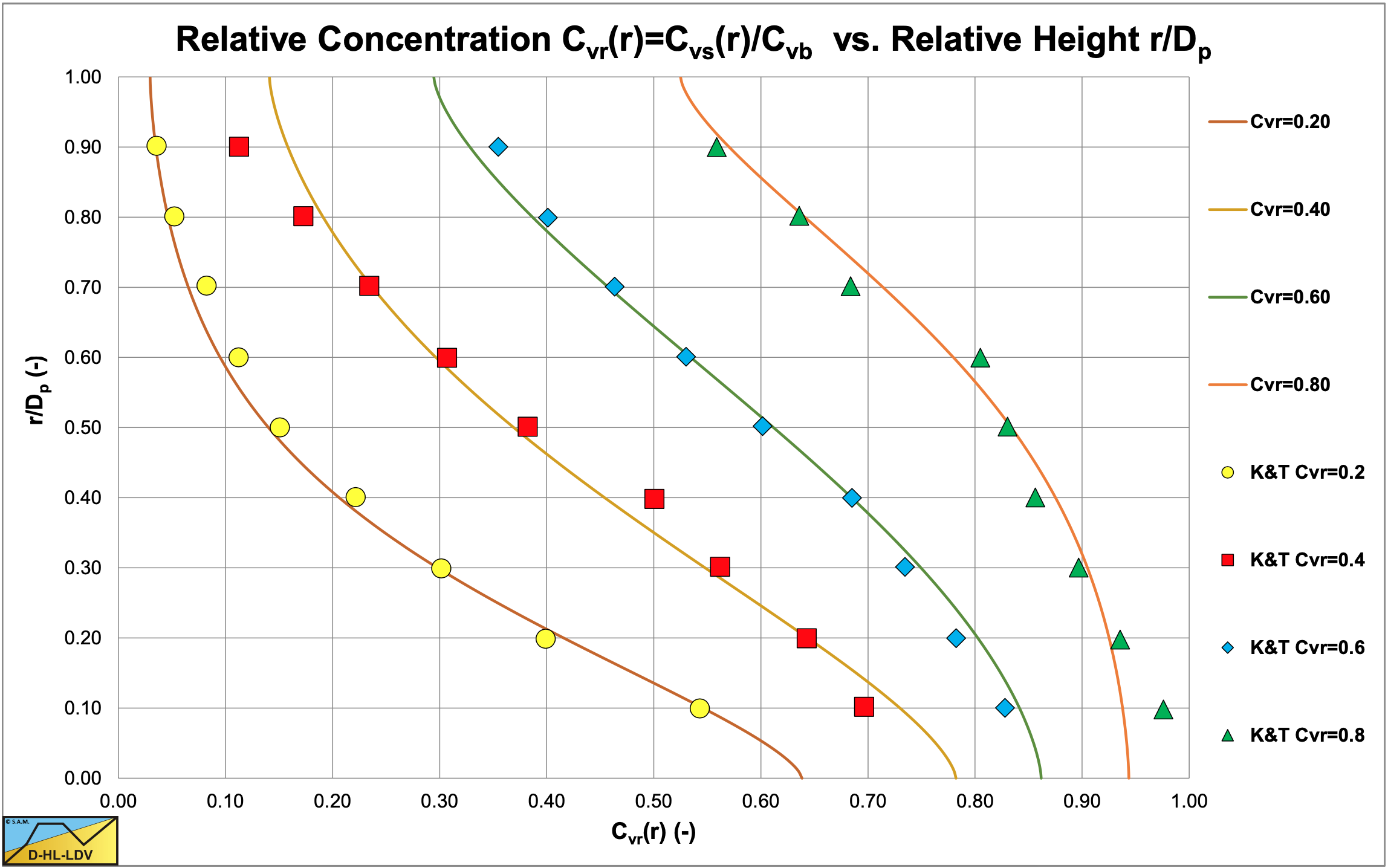
The data from Kaushal et al. (2005) with d=0.44 mm and D_p=0.0549 m are compared with the DHLLDV Framework. The maximum LDV for this sand and pipe diameter is about 2.5 m/s. The data points are at 3 m/s, so a bit above the LDV depending on the concentration, resulting in smaller concentrations at the bottom of the pipe.

Figure 6.23-1: Data from Kaushal et al. (2005) with local hindered settling.

6.23.3.1 Closed Ducts

Kaushal et al. (2002D) made the model applicable for a rectangular ducts, giving:

\[\ \begin{array}{left} \varepsilon_{\mathrm{s}}&=\beta_{\mathrm{sm}} \cdot \varepsilon_{\mathrm{m}}\\
\beta_{\mathrm{sm}}&=1+0.09322 \cdot \mathrm{e}^{5.5423 \cdot \frac{\mathrm{C}_{\mathrm{vs}}}{\mathrm{C}_{\mathrm{vb}}}}\end{array}\]

For the liquid eddy momentum diffusivity they used the equations suggested by Brooks & Berggren (1944):

\[\ \begin{array}{lll}\varepsilon_{\mathrm{m}}=\kappa \cdot \mathrm{u}_{*} \cdot \mathrm{H} \cdot \frac{\mathrm{z}}{\mathrm{H}} \cdot\left(1-\frac{2 \cdot \mathrm{z}}{\mathrm{H}}\right) & \text { for } & 0 \leq \frac{\mathrm{z}}{\mathrm{H}} \leq 0.337 \\ \varepsilon_{\mathrm{m}}=0.11 \cdot \mathrm{\kappa} \cdot \mathrm{u}_{*} \cdot \mathrm{H} & \text { for } & 0.337 \leq \frac{\mathrm{z}}{\mathrm{H}} \leq 0.663 \\ \varepsilon_{\mathrm{m}}=\kappa \cdot \mathrm{u}_{*} \cdot \mathrm{H} \cdot \frac{\mathrm{z}}{\mathrm{H}} \cdot\left(1-\frac{2 \cdot \mathrm{z}}{\mathrm{H}}\right) & \text { for } & 0.663 \leq \frac{\mathrm{z}}{\mathrm{H}} \leq 1.0\end{array}\]

6.23.3.2 Open Channel Flow

Seshadri et al. (2006) add equations for the liquid eddy momentum diffusivity for open channel flow:

\[\ \begin{array}{ll}\varepsilon_{\mathrm{m}}=2.5 \cdot \mathrm{\kappa} \cdot \mathrm{u}_{*} \cdot \mathrm{H} \cdot \frac{\mathrm{z}}{\mathrm{H}} & \text { for } \quad 0 \leq \frac{\mathrm{z}}{\mathrm{H}} \leq 0.1 \\ \varepsilon_{\mathrm{m}}=0.25 \cdot \mathrm{k} \cdot \mathrm{u}_{*} \cdot \mathrm{H} & \text { for } \quad 0.1 \leq \frac{\mathrm{z}}{\mathrm{H}} \leq 1.0\end{array}\]

6.23.4 Discussion & Conclusions

Up to 2014 the Kaushal & Tomita (2002B) model for the determination of the concentration profile is the most sophisticated model available. The prediction of concentration profiles with experimental data is very good. However there are some questions about the application of the Wasp et al. (1977) model:

1. The Wasp et al. (1977) criterion for the determination of the suspended load fraction is based on the original Wasp model. Does this criterion still hold if the concentration profile is determined in another way?
2. Kaushal & Tomita (2002B) use the particle drag coefficient C_D in the equation for the heterogeneous regime and not the particle Froude number C_x as used in the original Durand & Condolios (1952) equation. This may give a different result, especially at different solids submerged densities.
3. For very low line speeds, the model behaves like the Durand & Condolios (1952) model, not including sliding bed behavior. The assumption that the Durand & Condolios (1952) model describes bed behavior is incorrect. Durand & Condolios (1952) describe heterogeneous behavior, which is already a combination of bed behavior and suspended flow behavior.
4. For very high line speeds the model behaves like the Darcy Weisbach equation for pure carrier liquid. The model does not have asymptotic behavior towards the ELM model, due to the implementation of the Fanning friction factor.
5. The Hunt equation already takes into account some hindered settling effect because of the upwards liquid velocity. Is it correct to use the full hindered settling equation in the model, or should the power be 1 less?

6.23.5 Nomenclature Kaushal & Tomita Models

a	Coefficient Fanning friction factor	-
b	Coefficient Fanning friction factor	-
c ​​​​​​​	Coefficient Fanning friction factor	-
Cvs	Spatial volumetric concentration	-
Cvs,j	Spatial volumetric concentration, j^th fraction	-
Cvs,v	Spatial volumetric concentration vehicle (homogeneous fraction)	-
Cvs,v,j	Spatial volumetric concentration vehicle (homogeneous fraction), j^th fraction	-
Cvs,Du	Spatial volumetric concentration Durand fraction (heterogeneous fraction)	-
Cvc,Du,j	Spatial volumetric concentration Durand fraction (heterogeneous fraction), j^th fraction	-
Ctop	Spatial volumetric concentration at 92% of the pipe diameter, from the bottom of the pipe	-
Ctop,j	Spatial volumetric concentration at 92% of the pipe diameter, from the bottom of the pipe, j^th fraction	-
Ccenter	Spatial volumetric concentration at 50% of the pipe diameter, from the bottom of the pipe	-
Ccenter,j	Spatial volumetric concentration at 50% of the pipe diameter, from the bottom of the pipe, j^th fraction	-
Cvb	Spatial volumetric concentration bed	-
CvB	Spatial volumetric concentration bottom of pipe	-
Cvm	Concentration by weight	-
CD	Particle drag coefficient	-
CD,j	Particle drag coefficient j^th fraction	-
Cx	Durand & Condolios reversed particle Froude number squared	-
Cx,j	Durand & Condolios reversed particle Froude number squared j^th fraction	-
d	Particle diameter	-
dj	Particle diameter j^th fraction	m
dm	Mean particle diameter, Kaushal & Tomita	m
dmw	Weighed mean particle diameter, Kaushal & Tomita	m
Dp	Pipe diameter	m
E	Karabelas factor	-
Erhg	Relative excess hydraulic gradient	-
fm	Fanning friction factor mixture, Kaushal & Tomita	-
g	Gravitational constant 9.81 m/s^2	m/s^2
G	Karabelas factor	-
im	Hydraulic gradient mixture	-
ibed	Hydraulic gradient bed, Kaushal & Tomita	-
ibed,j	Hydraulic gradient bed j^th fraction, Kaushal & Tomita	-
ivehicle, ilv	Hydraulic gradient vehicle	-
iDu	Hydraulic gradient heterogeneous transport	-
iDu,j	Hydraulic gradient heterogeneous transport, contribution j^th fraction	-
itotal	Total hydraulic gradient, homogeneous plus heterogeneous	-
j	Fraction number	-
ΔL	Length of pipeline	m
LDV	Limit Deposit Velocity	m/s
n	Number of fractions	-
R	Pipe radius	m
Re	Reynolds number	-
Rem	Reynolds number	-
Rsd	Relative submerged density solids in pure liquid	-
u*	Friction velocity	m/s
vls	Line speed	m/s
vt	Terminal settling velocity in pure liquid	m/s
vt,j	Terminal settling velocity in pure liquid of the j^th fraction
vtv	Terminal settling velocity in the vehicle	m/s
vtv,j	Terminal settling velocity in the vehicle of the j^th fraction	m/s
z	Vertical coordinate in pipe	m
βsm, ζ	Relation sediment diffusivity – eddy momentum diffusivity	-
ε	Pipe wall roughness	m
εs	Sediment diffusivity	m/s
εm	Eddy momentum diffusivity	m/s
κ	Von Karman constant, about 0.4	-
λl	Darcy Weisbach friction factor based on liquid properties	-
λm	Darcy Weisbach friction factor mixture, Kaushal & Tomita	-
ρl	Density liquid	ton/m^3
ρs	Density solids	ton/m^3
ρm	Density mixture	ton/m^3
ρv	Density vehicle	ton/m^3
σg	PSD grading coefficient, Kaushal & Tomita	-
\(\ v_{\mathrm{l}}\)	Kinematic viscosity pure liquid	m^2/s