
6.22: The SRC Model
- Page ID
- 31441

\( \newcommand{\vecs}[1]{\overset { \scriptstyle \rightharpoonup} {\mathbf{#1}} } \)
\( \newcommand{\vecd}[1]{\overset{-\!-\!\rightharpoonup}{\vphantom{a}\smash {#1}}} \)
\( \newcommand{\id}{\mathrm{id}}\) \( \newcommand{\Span}{\mathrm{span}}\)
( \newcommand{\kernel}{\mathrm{null}\,}\) \( \newcommand{\range}{\mathrm{range}\,}\)
\( \newcommand{\RealPart}{\mathrm{Re}}\) \( \newcommand{\ImaginaryPart}{\mathrm{Im}}\)
\( \newcommand{\Argument}{\mathrm{Arg}}\) \( \newcommand{\norm}[1]{\| #1 \|}\)
\( \newcommand{\inner}[2]{\langle #1, #2 \rangle}\)
\( \newcommand{\Span}{\mathrm{span}}\)
\( \newcommand{\id}{\mathrm{id}}\)
\( \newcommand{\Span}{\mathrm{span}}\)
\( \newcommand{\kernel}{\mathrm{null}\,}\)
\( \newcommand{\range}{\mathrm{range}\,}\)
\( \newcommand{\RealPart}{\mathrm{Re}}\)
\( \newcommand{\ImaginaryPart}{\mathrm{Im}}\)
\( \newcommand{\Argument}{\mathrm{Arg}}\)
\( \newcommand{\norm}[1]{\| #1 \|}\)
\( \newcommand{\inner}[2]{\langle #1, #2 \rangle}\)
\( \newcommand{\Span}{\mathrm{span}}\) \( \newcommand{\AA}{\unicode[.8,0]{x212B}}\)
\( \newcommand{\vectorA}[1]{\vec{#1}} % arrow\)
\( \newcommand{\vectorAt}[1]{\vec{\text{#1}}} % arrow\)
\( \newcommand{\vectorB}[1]{\overset { \scriptstyle \rightharpoonup} {\mathbf{#1}} } \)
\( \newcommand{\vectorC}[1]{\textbf{#1}} \)
\( \newcommand{\vectorD}[1]{\overrightarrow{#1}} \)
\( \newcommand{\vectorDt}[1]{\overrightarrow{\text{#1}}} \)
\( \newcommand{\vectE}[1]{\overset{-\!-\!\rightharpoonup}{\vphantom{a}\smash{\mathbf {#1}}}} \)
\( \newcommand{\vecs}[1]{\overset { \scriptstyle \rightharpoonup} {\mathbf{#1}} } \)
\( \newcommand{\vecd}[1]{\overset{-\!-\!\rightharpoonup}{\vphantom{a}\smash {#1}}} \)
\(\newcommand{\avec}{\mathbf a}\) \(\newcommand{\bvec}{\mathbf b}\) \(\newcommand{\cvec}{\mathbf c}\) \(\newcommand{\dvec}{\mathbf d}\) \(\newcommand{\dtil}{\widetilde{\mathbf d}}\) \(\newcommand{\evec}{\mathbf e}\) \(\newcommand{\fvec}{\mathbf f}\) \(\newcommand{\nvec}{\mathbf n}\) \(\newcommand{\pvec}{\mathbf p}\) \(\newcommand{\qvec}{\mathbf q}\) \(\newcommand{\svec}{\mathbf s}\) \(\newcommand{\tvec}{\mathbf t}\) \(\newcommand{\uvec}{\mathbf u}\) \(\newcommand{\vvec}{\mathbf v}\) \(\newcommand{\wvec}{\mathbf w}\) \(\newcommand{\xvec}{\mathbf x}\) \(\newcommand{\yvec}{\mathbf y}\) \(\newcommand{\zvec}{\mathbf z}\) \(\newcommand{\rvec}{\mathbf r}\) \(\newcommand{\mvec}{\mathbf m}\) \(\newcommand{\zerovec}{\mathbf 0}\) \(\newcommand{\onevec}{\mathbf 1}\) \(\newcommand{\real}{\mathbb R}\) \(\newcommand{\twovec}[2]{\left[\begin{array}{r}#1 \\ #2 \end{array}\right]}\) \(\newcommand{\ctwovec}[2]{\left[\begin{array}{c}#1 \\ #2 \end{array}\right]}\) \(\newcommand{\threevec}[3]{\left[\begin{array}{r}#1 \\ #2 \\ #3 \end{array}\right]}\) \(\newcommand{\cthreevec}[3]{\left[\begin{array}{c}#1 \\ #2 \\ #3 \end{array}\right]}\) \(\newcommand{\fourvec}[4]{\left[\begin{array}{r}#1 \\ #2 \\ #3 \\ #4 \end{array}\right]}\) \(\newcommand{\cfourvec}[4]{\left[\begin{array}{c}#1 \\ #2 \\ #3 \\ #4 \end{array}\right]}\) \(\newcommand{\fivevec}[5]{\left[\begin{array}{r}#1 \\ #2 \\ #3 \\ #4 \\ #5 \\ \end{array}\right]}\) \(\newcommand{\cfivevec}[5]{\left[\begin{array}{c}#1 \\ #2 \\ #3 \\ #4 \\ #5 \\ \end{array}\right]}\) \(\newcommand{\mattwo}[4]{\left[\begin{array}{rr}#1 \amp #2 \\ #3 \amp #4 \\ \end{array}\right]}\) \(\newcommand{\laspan}[1]{\text{Span}\{#1\}}\) \(\newcommand{\bcal}{\cal B}\) \(\newcommand{\ccal}{\cal C}\) \(\newcommand{\scal}{\cal S}\) \(\newcommand{\wcal}{\cal W}\) \(\newcommand{\ecal}{\cal E}\) \(\newcommand{\coords}[2]{\left\{#1\right\}_{#2}}\) \(\newcommand{\gray}[1]{\color{gray}{#1}}\) \(\newcommand{\lgray}[1]{\color{lightgray}{#1}}\) \(\newcommand{\rank}{\operatorname{rank}}\) \(\newcommand{\row}{\text{Row}}\) \(\newcommand{\col}{\text{Col}}\) \(\renewcommand{\row}{\text{Row}}\) \(\newcommand{\nul}{\text{Nul}}\) \(\newcommand{\var}{\text{Var}}\) \(\newcommand{\corr}{\text{corr}}\) \(\newcommand{\len}[1]{\left|#1\right|}\) \(\newcommand{\bbar}{\overline{\bvec}}\) \(\newcommand{\bhat}{\widehat{\bvec}}\) \(\newcommand{\bperp}{\bvec^\perp}\) \(\newcommand{\xhat}{\widehat{\xvec}}\) \(\newcommand{\vhat}{\widehat{\vvec}}\) \(\newcommand{\uhat}{\widehat{\uvec}}\) \(\newcommand{\what}{\widehat{\wvec}}\) \(\newcommand{\Sighat}{\widehat{\Sigma}}\) \(\newcommand{\lt}{<}\) \(\newcommand{\gt}{>}\) \(\newcommand{\amp}{&}\) \(\definecolor{fillinmathshade}{gray}{0.9}\)Where the Wilson-GIW (1979) model as discussed in a previous chapter deals with a stationary or sliding bed layer (the lower layer) with a liquid layer above it (the upper layer), the model described here is made to cope with the complexities of industrial slurries. At the Saskatchewan Research Council (SRC) the model has been developed and improved over the years. The SRC model is the result of work carried out by Dr. C.A. Shook (University of Saskatchewan) and his associates at the Saskatchewan Research Council. The SRC model assumes that the suspended solids are distributed uniformly across the entire pipe and that the lower layer also contains the solids that contribute Coulombic friction. One will find an early version of the SRC model in in the Hydrotransport 10 proceedings, Shook et al. (1986). Later the model is discussed in the book of Shook & Roco (1991) and many other publications.
6.22.1 Continuity Equations
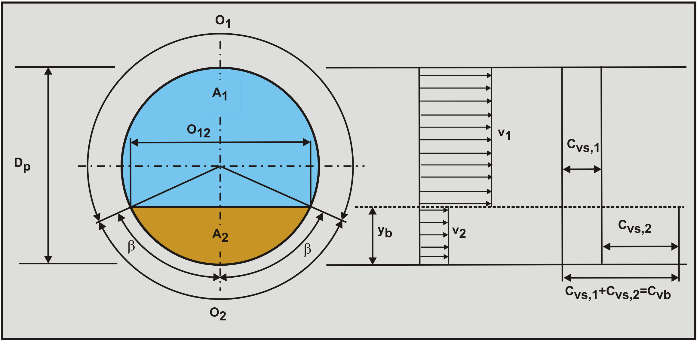
It should be mentioned that the model assumes suspension moving with the cross sectional average line speed vls over the full pipe cross section. The volumetric flow rate of mixture is:
\[\ \mathrm{v}_{\mathrm{l} \mathrm{s}} \cdot \mathrm{A}_{\mathrm{p}}=\mathrm{v}_{\mathrm{1}} \cdot \mathrm{A}_{\mathrm{1}}+\mathrm{v}_{\mathrm{2}} \cdot \mathrm{A}_{\mathrm{2}}\]
For the solids, neglecting local slip of the particles relative to the liquid, the flow rate resulting in the delivered concentration is:
\[\ \mathrm{v}_{\mathrm{l s}} \cdot \mathrm{A}_{\mathrm{p}} \cdot \mathrm{C}_{\mathrm{v t}}=\mathrm{v}_{\mathrm{l s}} \cdot \mathrm{A}_{\mathrm{p}} \cdot \mathrm{C}_{\mathrm{v s}, \mathrm{1}}+\mathrm{v}_{\mathrm{2}} \cdot \mathrm{A}_{\mathrm{2}} \cdot \mathrm{C}_{\mathrm{v s}, \mathrm{2}}\]
In the original model the concentration Cvs,1 was zero, so now a method must be employed to predict Cvs,1. In fact the so called contact load Cvs,c is determined first and from there the concentration Cvs,1. Physically Cvs,c represents the time averaged volumetric concentration contributing Coulombic friction to the flow. In terms of spatial volumetric concentration, the total spatial volumetric concentration consists of the suspended load concentration and the contact load concentration, so:
\[\ \mathrm{A}_{\mathrm{p}} \cdot \mathrm{C}_{\mathrm{v s}}=\mathrm{A}_{\mathrm{p}} \cdot \mathrm{C}_{\mathrm{v s}, \mathrm{1}}+\mathrm{A}_{\mathrm{p}} \cdot \mathrm{C}_{\mathrm{v s}, \mathrm{c}}=\mathrm{A}_{\mathrm{p}} \cdot \mathrm{C}_{\mathrm{v s}, \mathrm{1}}+\mathrm{A}_{\mathrm{2}} \cdot \mathrm{C}_{\mathrm{v s}, \mathrm{2}}\]
6.22.2 Concentrations
The SRC model is based on spatial volumetric concentrations. Delivered volumetric concentrations are an output of the model. The total spatial volumetric concentration is according to equation (6.22-3):
\[\ \mathrm{C}_{\mathrm{v s}}=\mathrm{C}_{\mathrm{v s}, \mathrm{1}}+\mathrm{C}_{\mathrm{v s}, \mathrm{c}}=\mathrm{C}_{\mathrm{v s}, \mathrm{1}}+\frac{\mathrm{A}_{2}}{\mathrm{A}_{\mathrm{p}}} \cdot \mathrm{C}_{\mathrm{v s}, \mathrm{2}} \quad\text{ with: }\quad \frac{\mathrm{A}_{2}}{\mathrm{A}_{\mathrm{p}}}=\frac{\mathrm{C}_{\mathrm{v s}, \mathrm{c}}}{\mathrm{C}_{\mathrm{v s}, \mathrm{2}}}=\frac{\mathrm{C}_{\mathrm{v s}, \mathrm{c}}}{\mathrm{C}_{\mathrm{v b}}-\mathrm{C}_{\mathrm{v s}}+\mathrm{C}_{\mathrm{v s}, \mathrm{c}}}\]
The spatial contact load concentration is now:
\[\ \mathrm{C_{\mathrm{vs}, \mathrm{c}}=\frac{\mathrm{A}_{2}}{\mathrm{A}_{\mathrm{p}}} \cdot \mathrm{C}_{\mathrm{vs}, 2} \quad\text{ and }\quad \mathrm{C}_{\mathrm{vs}, 2}=\frac{\mathrm{A}_{\mathrm{p}}}{\mathrm{A}_{2}} \cdot \mathrm{C}_{\mathrm{vs}, \mathrm{c}}}\]
Shook & Roco (1991) mention two equations to determine the contact load concentration Cvc,c.
Their first equation:
\[\ \mathrm{\frac{C_{v s, c}}{C_{v s}}=e^{-0.124 \cdot A r^{-0.061} \cdot\left(\frac{v_{ls}^{2}}{g \cdot d}\right)^{-0.028} \cdot\left(\frac{d}{D_{p}}\right)^{-0.431} \cdot R_{s d}^{-0.272}}}\]
Their second equation:
\[\ \mathrm{\frac{C_{v s, c}}{C_{v s}}=e^{-0.122 \cdot A r^{-0.12} \cdot\left(\frac{v_{l s}}{v_{l s, ld v}}\right)^{0.3} \cdot\left(\frac{d}{D_{p}}\right)^{-0.51} \cdot R_{s d}^{-0.255}}}\]
Shook & Roco (1991), based these equations on the particle Archimedes number:
\[\ \mathrm{Ar}=\frac{4 \cdot \mathrm{g} \cdot \mathrm{d}^{3} \cdot \mathrm{R}_{\mathrm{sd}}}{3 \cdot v_{\mathrm{l}}^{2}}\]
Note that in the first equation only the line speed vls plays a role. In the second equation the ratio line speed vls to Limit Deposit Velocity vls,ldv plays a role.
6.22.3 The Mixture Densities
Shook & Roco (1991) assume that the particles in contact load are carried by a mixture formed by the carrier liquid and the particles in suspended load. In the upper layer there are only particles in suspended load, giving the mixture in the upper layer a density of:
\[\ \rho_{\mathrm{m} 1}=\rho_{\mathrm{l}} \cdot\left(1-\mathrm{C}_{\mathrm{vs}, 1}\right)+\rho_{\mathrm{s}} \cdot \mathrm{C}_{\mathrm{vs}, 1}=\rho_{\mathrm{l}}+\mathrm{C}_{\mathrm{vs}, 1} \cdot\left(\rho_{\mathrm{s}}-\rho_{\mathrm{l}}\right)\]
They suppose that the contact load particles are carried by the mixture of the carrier liquid and the suspended load particles. To determine this buoyancy effect, one has to take into account that the available volume for the mixture equals the total bed volume minus the volume occupied by the particles, giving:
\[\ \rho_{\mathrm{m} 2} \cdot\left(1-\mathrm{C}_{\mathrm{vs}, 2}\right)=\rho_{\mathrm{l}} \cdot\left(1-\mathrm{C}_{\mathrm{vs}, 1}-\mathrm{C}_{\mathrm{vs}, 2}\right)+\rho_{\mathrm{s}} \cdot \mathrm{C}_{\mathrm{vs}, 1}\]
The mixture density in the lower layer ρm2 is now:
\[\ \rho_{\mathrm{m} 2}=\frac{\rho_{\mathrm{l}} \cdot\left(1-\mathrm{C}_{\mathrm{vs}, 1}-\mathrm{C}_{\mathrm{vs}, 2}\right)+\rho_{\mathrm{s}} \cdot \mathrm{C}_{\mathrm{vs}, 1}}{\left(1-\mathrm{C}_{\mathrm{vs}, 2}\right)}=\rho_{\mathrm{l}}+\frac{\mathrm{C}_{\mathrm{vs}, 1}}{\left(1-\mathrm{C}_{\mathrm{vs}, 2}\right)} \cdot\left(\rho_{\mathrm{s}}-\rho_{\mathrm{l}}\right)\]
6.22.4 Pressure Gradients & Shear Stresses
The pressure gradient \(-Δp/ΔL\) on the liquid above the bed opposes the friction forces due to shear stresses between the liquid and the pipe wall and the liquid and the bed:
\[\ -\frac{\Delta \mathrm{p}}{\Delta \mathrm{L}}=\frac{\tau_{1,\mathrm{l}} \cdot \mathrm{O}_{1}+\tau_{12,\mathrm{l}} \cdot \mathrm{O}_{12}}{\mathrm{A}_{1}}\]
The pressure gradient \(-Δp/ΔL\) on the bed is opposes the friction forces due to shear stresses between the bed and the pipe wall (sliding friction and viscous friction) minus the driving force due to the friction between the liquid in the upper layer and the bed interface:
\[\ -\frac{\Delta \mathrm{p}}{\Delta \mathrm{L}}=\frac{\tau_{2, \mathrm{sf}} \cdot \mathrm{O}_{2}+\tau_{2,\mathrm{l}} \cdot \mathrm{O}_{2}-\tau_{12,\mathrm{l}} \cdot \mathrm{O}_{12}}{\mathrm{A}_{2}}\]
For the whole pipe cross section this gives the shear forces due to shear stresses between the liquid in the upper layer and the pipe wall and the shear stresses between the bed and the pipe wall. The shear stresses between the upper layer and the lower layer (the bed) are internal and do not play a role here:
\[\ -\frac{\Delta \mathrm{p}}{\Delta \mathrm{L}}=\frac{\tau_{2, \mathrm{sf}} \cdot \mathrm{0}_{2}+\tau_{2,\mathrm{l}} \cdot \mathrm{O}_{2}+\tau_{1,\mathrm{l}} \cdot \mathrm{0}_{1}}{\mathrm{A}_{\mathrm{p}}}\]
The shear stress \(\ \mathrm{\tau}_{1,1}\) on the pipe wall can be evaluated with the well-known Darcy Weisbach equation:
\[\ \tau_{1,\mathrm{l}}=\frac{\lambda_{1}}{4} \cdot \frac{1}{2} \cdot \rho_{\mathrm{m} 1} \cdot \mathrm{v}_{1}^{2} \quad\text{ with: }\quad \lambda_{1}=\frac{1.325}{\left(\ln \left(\frac{0.27 \cdot \varepsilon}{\mathrm{D}_{\mathrm{H}}}+\frac{5.75}{\mathrm{Re}^{0.9}}\right)\right)^{2}}\quad\text{ and }\quad \operatorname{Re}=\frac{\mathrm{v}_{1} \cdot \mathrm{D}_{\mathrm{H}}}{v_{\mathrm{l}}}\]
In their book Shook & Roco (1991) use the cross section average line speed vls and the pipe diameter Dp in the above equation instead of the velocity in the upper layer v1 and the hydraulic diameter DH of the cross section of the upper layer.
For the flow between the liquid in the bed and the pipe wall, the shear stress between the liquid and the pipe wall is:
\[\ \tau_{2,\mathrm{l}}=\frac{\lambda_{1}}{4} \cdot \frac{1}{2} \cdot \rho_{\mathrm{m} 2} \cdot \mathrm{v}_{2}^{2}\]
For the flow in the restricted area, the shear stress between the liquid and the bed is:
\[\ \tau_{12,\mathrm{l}}=\frac{\lambda_{12}}{4} \cdot \frac{1}{2} \cdot \rho_{\mathrm{l}} \cdot\left(\mathrm{v_{1}-v_{2}}\right)^{2} \quad\text{ with: }\quad \lambda_{12}=\frac{\alpha \cdot 1.325}{\left(\ln \left(\frac{0.27 \cdot \mathrm{d}}{\mathrm{D}_{\mathrm{H}}}+\frac{5.75}{\mathrm{Re}^{0.9}}\right)\right)^{2}} \quad\text{ and }\quad \mathrm{Re}=\frac{\mathrm{v}_{1} \cdot \mathrm{D}_{\mathrm{H}}}{v_{\mathrm{l}}}\]
The factor α as used by Shook & Roco (1991) is 2.
6.22.5 The Sliding Friction
In order to use the original liquid density in the sliding friction equation, first the equation of the sliding friction of the bed with the pipe wall has to be written in terms of the new mixture/liquid density ρm2:
\[\ \tau_{2, \mathrm{sf}}=\frac{\mu_{\mathrm{sf}} \cdot \mathrm{g} \cdot\left(\rho_{\mathrm{s}}-\rho_{\mathrm{m} 2}\right) \cdot \mathrm{C}_{\mathrm{vs}, 2} \cdot \mathrm{A}_{\mathrm{p}}}{\beta \cdot \mathrm{D}_{\mathrm{p}}} \cdot \frac{2 \cdot(\sin (\beta)-\beta \cdot \cos (\beta))}{\pi}\]
The concentration used in this equation is the concentration of the contact load particles in the bed. For the difference between the solids density ρs and the mixture density ρm2 we can write:
\[\ \left(\rho_{\mathrm{s}}-\rho_{\mathrm{m} 2}\right)=\frac{\rho_{\mathrm{s}} \cdot\left(1-\mathrm{C}_{\mathrm{vs}, 2}\right)}{\left(1-\mathrm{C}_{\mathrm{vs}, 2}\right)}-\frac{\rho_{\mathrm{l}} \cdot\left(1-\mathrm{C}_{\mathrm{vs}, 1}-\mathrm{C}_{\mathrm{vs}, 2}\right)+\rho_{\mathrm{s}} \cdot \mathrm{C}_{\mathrm{vs}, 1}}{\left(1-\mathrm{C}_{\mathrm{vs}, 2}\right)}\]
Rewriting gives:
\[\ \begin{array}{left} \left(\rho_{\mathrm{s}}-\rho_{\mathrm{m} 2}\right) &=\frac{\rho_{\mathrm{s}} \cdot\left(1-\mathrm{C}_{\mathrm{vs}, 1}-\mathrm{C}_{\mathrm{vs}, 2}\right)-\rho_{\mathrm{l}} \cdot\left(1-\mathrm{C}_{\mathrm{vs}, 1}-\mathrm{C}_{\mathrm{vs}, 2}\right)}{\left(1-\mathrm{C}_{\mathrm{vs}, 2}\right)} \\ &=\left(\rho_{\mathrm{s}}-\rho_{\mathrm{l}}\right) \cdot \frac{\left(1-\mathrm{C}_{\mathrm{vs}, 1}-\mathrm{C}_{\mathrm{vs}, 2}\right)}{\left(1-\mathrm{C}_{\mathrm{vs}, 2}\right)} \end{array}\]
Shook & Roco (1991) add the effect of the suspended solids reducing the force transmitted to the wall, due to the buoyant effect on the contact load particles and assuming only the concentration Cvs,2 results in contact with the pipe wall and thus sliding friction, giving:
\[\ \tau_{2, \mathrm{sf}}=\frac{\mu_{\mathrm{sf}} \cdot \rho_{\mathrm{l}} \cdot \mathrm{g} \cdot \mathrm{R}_{\mathrm{sd}} \cdot \mathrm{C}_{\mathrm{v s}, \mathrm{2}} \cdot \mathrm{A}_{\mathrm{p}}}{\beta \cdot \mathrm{D}_{\mathrm{p}}} \cdot \frac{2 \cdot(\sin (\beta)-\beta \cdot \cos (\beta))}{\pi} \cdot \frac{\left(1-\mathrm{C}_{\mathrm{v s}, \mathrm{1}}-\mathrm{C}_{\mathrm{v s}, 2}\right)}{\left(1-\mathrm{C}_{\mathrm{v s}, 2}\right)}\]
Gillies (1993) also uses this approach. When the suspension concentration Cvs,1 equals zero, the Wilson et al. (1992) solution is found, with Cvs,2=Cvb. A value of 0.6 is mentioned for Cvb and a value of 0.5 is mentioned for μsf.
\[\ \tau_{2, \mathrm{sf}}=\frac{\mu_{\mathrm{sf}} \cdot \rho_{\mathrm{l}} \cdot \mathrm{g} \cdot \mathrm{R}_{\mathrm{sd}} \cdot \mathrm{C}_{\mathrm{vb}} \cdot \mathrm{A}_{\mathrm{p}}}{\beta \cdot \mathrm{D}_{\mathrm{p}}} \cdot \frac{2 \cdot(\sin (\beta)-\beta \cdot \cos (\beta))}{\pi}\]
The model assumes that the lower layer does contain particles suspended by turbulence. These suspended particles contribute buoyancy helping to reduce the immersed weight of the supported particles. Small particles in the bed become part of the bed and transmit the submerged gravity forces by interparticle contact. Only very small particles are assumed to form a homogeneous carrier liquid with an adjusted viscosity and density. In the case of a uniform particle size distribution (all the particles have the same size), equations (6.22-6), (6.22-7) and (6.22-43) will give a contact load and suspended load fraction Cvs,c and Cvs,1. However, the suspended load particles in the bed are the same sized particles as the contact load particles. So a portion of the same sized particles is carrying part of the submerged weight of the other portion of the same sized particles. In the case of a very graded sand, one may assume that the suspended load particles consist of the fine portion of the PSD and the contact load particles of the coarse part of the PSD. Shook & Roco (1991) use different equations for the determination of the Darcy Weisbach friction factor. Here the Swamee Jain (1976) equation is used. In order to find the equilibrium of forces on the bed (the lower layer) an iterative algorithm has to be used. Outputs are the pressure gradient and the delivered concentration, also resulting in a slip ratio.
The resulting pressure can be determined by:
\[\ \Delta \mathrm{p}=\frac{\Delta \mathrm{F}}{\mathrm{A}_{\mathrm{p}}}=\frac{\left(\tau_{1,\mathrm{}1} \cdot(\pi-\beta)+\tau_{2,1} \cdot \beta+\tau_{2, \mathrm{sf}} \cdot \beta\right) \cdot \mathrm{D}_{\mathrm{p}} \cdot \Delta \mathrm{L}}{\mathrm{A}_{\mathrm{p}}}\]
Substituting the shear stresses gives:
\[\ \Delta \mathrm{p}=\frac{\left(\begin{array}{c}\frac{\lambda_{1}}{4} \cdot \frac{1}{2} \cdot \rho_{\mathrm{m} 1} \cdot \mathrm{v}_{1}^{2} \cdot(\pi-\beta)+\frac{\lambda_{1}}{4} \cdot \frac{1}{2} \cdot \rho_{\mathrm{m} 2} \cdot \mathrm{v}_{2}^{2} \cdot \beta \\ +\frac{\mu_{\mathrm{sf}} \cdot \rho_{\mathrm{l}} \cdot \mathrm{g} \cdot \mathrm{R}_{\mathrm{sd}} \cdot \mathrm{C}_{\mathrm{vs}, 2} \cdot \mathrm{A}_{\mathrm{p}}}{\beta \cdot \mathrm{D}_{\mathrm{p}}} \cdot \frac{2 \cdot(\sin (\beta)-\beta \cdot \cos (\beta))}{\pi} \cdot \frac{\left(1-\mathrm{C}_{\mathrm{vs}, 1}-\mathrm{C}_{\mathrm{vs}, 2}\right)}{\left(1-\mathrm{C}_{\mathrm{vs}, 2}\right)} \cdot \beta\end{array}\right) \cdot \mathrm{D}_{\mathrm{p}} \cdot \Delta \mathrm{L}}{\mathrm{A_p}} \]
This can be simplified to:
\[\ \begin{array}{left} \Delta \mathrm{p}=& \lambda_{\mathrm{1}} \cdot \frac{\Delta \mathrm{L}}{\mathrm{D}_{\mathrm{p}}} \cdot\left(\frac{\mathrm{1}}{2} \cdot \rho_{\mathrm{m} 1} \cdot \mathrm{v}_{\mathrm{1}}^{2} \cdot \frac{(\pi-\beta)}{\pi}+\frac{\mathrm{1}}{2} \cdot \rho_{\mathrm{m} 2} \cdot \mathrm{v}_{\mathrm{2}}^{2} \cdot \frac{\beta}{\pi}\right) \\ &+\mu_{\mathrm{sf}} \cdot \rho_{\mathrm{l}} \cdot \mathrm{g} \cdot \mathrm{R}_{\mathrm{s d}} \cdot \mathrm{C}_{\mathrm{v s}, \mathrm{2}} \cdot \frac{\mathrm{2} \cdot(\sin (\beta)-\beta \cdot \cos (\beta))}{\pi} \cdot \frac{\left(\mathrm{1}-\mathrm{C}_{\mathrm{v s}, \mathrm{1}}-\mathrm{C}_{\mathrm{v s}, \mathrm{2}}\right)}{\left(\mathrm{1}-\mathrm{C}_{\mathrm{v s}, \mathrm{2}}\right)} \cdot \Delta \mathrm{L} \end{array}\]
The hydraulic gradient of the mixture is now:
\[\ \mathrm{i}_{\mathrm{m}}=\frac{\Delta \mathrm{p}}{\rho_{\mathrm{l}} \cdot \mathrm{g} \cdot \Delta \mathrm{L}}=\frac{\lambda_{1}}{2 \cdot \mathrm{g} \cdot \mathrm{D}_{\mathrm{p}}} \cdot\left(\begin{array}{c}\frac{\rho_{\mathrm{l}}+\mathrm{C}_{\mathrm{v} \mathrm{s}, \mathrm{1}} \cdot\left(\rho_{\mathrm{s}}-\rho_{\mathrm{l}}\right)}{\rho_{\mathrm{l}}} \cdot \mathrm{v}_{1}^{2} \cdot \frac{(\pi-\beta)}{\pi} \\ +\frac{\rho_{\mathrm{l}}+\frac{\mathrm{C}_{\mathrm{v} \mathrm{s}, \mathrm{1}}}{\left(1-\mathrm{C}_{\mathrm{v s}, 2}\right)} \cdot\left(\rho_{\mathrm{s}}-\rho_{\mathrm{l}}\right)}{\rho_{\mathrm{l}}} \cdot \mathrm{v}_{2}^{2} \cdot \frac{\beta}{\pi}\end{array}\right)+\mathrm{\mu_{sf}\cdot R_{sd}\cdot C_{vs,2}\cdot \frac{2 \cdot (sin(\beta)-\beta \cdot cos(\beta))}{\pi}}\cdot \mathrm{\frac{(1-c_{vs,1}-C_{vs,2})}{(1-C_{vs,2})}}\]
This can be simplified to:
\[\ \mathrm{i}_{\mathrm{m}}=\frac{\lambda_{1}}{\mathrm{2} \cdot \mathrm{g} \cdot \mathrm{D}_{\mathrm{p}}} \cdot\left(\begin{array}{c}\left(1+\mathrm{C}_{\mathrm{v s}, 1} \cdot \mathrm{R}_{\mathrm{sd}}\right) \cdot \mathrm{v}_{1}^{2} \cdot \frac{(\pi-\beta)}{\pi} \\ +(\mathrm{1 + \frac { \mathrm { C } _ { \mathrm { v s } , \mathrm { 1 } } } { ( 1 - \mathrm { C } _ { \mathrm { v s } , 2 } ) } \cdot \mathrm { R } _ { \mathrm { sd } }}) \cdot \mathrm{v}_{2}^{2} \cdot \frac{\beta}{\pi}\end{array}\right) + \mathrm{\mu_{sf}\cdot R_{sd}\cdot C_{vs,2}\cdot \frac{2\cdot (sin(\beta)-\beta \cdot cos(\beta))}{\pi}\cdot \frac{(1-C_{vs,1}-C_{vs,2})}{(1-C_{vs,2})}}\]
Or:
\[\ \mathrm{i}_{\mathrm{m}}=\frac{\lambda_{1}}{\mathrm{2} \cdot \mathrm{g} \cdot \mathrm{D}_{\mathrm{p}}} \cdot\left(\begin{array}{l}\left(\mathrm{v}_{1}^{2} \cdot \frac{(\pi-\beta)}{\pi}+\mathrm{v}_{2}^{2} \cdot \frac{\beta}{\pi}\right) \\ \left.+\mathrm{C}_{\mathrm{v s}, \mathrm{1}} \cdot \mathrm{R}_{\mathrm{s d}} \cdot \mathrm{v}_{1}^{2} \cdot \frac{(\pi-\beta)}{\pi}+\frac{\mathrm{C}_{\mathrm{v} \mathrm{s}, \mathrm{1}}}{\left(1-\mathrm{C}_{\mathrm{v s}, 2}\right)} \cdot \mathrm{R}_{\mathrm{sd}} \cdot \mathrm{v}_{2}^{2} \cdot \frac{\beta}{\pi}\right)\end{array}\right)+\mathrm{\mu_{sf}\cdot R_{sd}\cdot C_{vs,2}\cdot \frac{2 \cdot (sin(\beta)-\beta\cdot cos(\beta))}{\pi}}\cdot \mathrm{\frac{(1-C_{vs,1}-C_{vs,2})}{(1-C_{vs,2})}}\]
Assuming that the first term between the brackets almost equals the line speed squared, this gives:
\[\ \begin{array}{left} \mathrm{i}_{\mathrm{m}}=& \frac{\lambda_{\mathrm{1}}}{\mathrm{2} \cdot \mathrm{g} \cdot \mathrm{D}_{\mathrm{p}}} \cdot\left(\mathrm{v}_{\mathrm{l} \mathrm{s}}^{\mathrm{2}}+\mathrm{C}_{\mathrm{v} \mathrm{s}, \mathrm{1}} \cdot \mathrm{R}_{\mathrm{s} \mathrm{d}} \cdot \mathrm{v}_{\mathrm{1}}^{2} \cdot \frac{(\pi-\beta)}{\pi}+\frac{\mathrm{C}_{\mathrm{v s}, \mathrm{1}}}{\left(\mathrm{1}-\mathrm{C}_{\mathrm{v} \mathrm{s}, \mathrm{2}}\right)} \cdot \mathrm{R}_{\mathrm{s} \mathrm{d}} \cdot \mathrm{v}_{\mathrm{2}}^{2} \cdot \frac{\beta}{\pi}\right) \\ &+\mu_{\mathrm{s} \mathrm{f}} \cdot \mathrm{R}_{\mathrm{s} \mathrm{d}} \cdot \mathrm{C}_{\mathrm{v s}, \mathrm{2}} \cdot \frac{\mathrm{2} \cdot(\sin (\beta)-\beta \cdot \cos (\beta))}{\pi} \cdot \frac{\left(1-\mathrm{C}_{\mathrm{v s}, \mathrm{1}}-\mathrm{C}_{\mathrm{v} \mathrm{s}, \mathrm{2}}\right)}{\left(\mathrm{1}-\mathrm{C}_{\mathrm{v s}, \mathrm{2}}\right)} \end{array}\]
In terms of the relative excess hydraulic gradient this can be written as:
\[\ \begin{array}{left} \mathrm{E}_{\mathrm{r h g}} &=\frac{\mathrm{i}_{\mathrm{m}}-\mathrm{i}_{\mathrm{l}}}{\mathrm{R}_{\mathrm{s} \mathrm{d}} \cdot \mathrm{C}_{\mathrm{v} \mathrm{s}}}=\frac{\lambda_{\mathrm{1}}}{\mathrm{2} \cdot \mathrm{g} \cdot \mathrm{D}_{\mathrm{p}}} \cdot\left(\frac{\mathrm{C}_{\mathrm{v s}, \mathrm{1}}}{\mathrm{C}_{\mathrm{v s}}} \cdot \mathrm{v}_{\mathrm{1}}^{2} \cdot \frac{(\pi-\beta)}{\pi}+\frac{\mathrm{C}_{\mathrm{v s}, \mathrm{1}}}{\left(1-\mathrm{C}_{\mathrm{v s}, \mathrm{2}}\right) \cdot \mathrm{C}_{\mathrm{v} \mathrm{s}}} \cdot \mathrm{v}_{\mathrm{2}}^{2} \cdot \frac{\beta}{\pi}\right) \\+& \mu_{\mathrm{sf}} \cdot \frac{\mathrm{C}_{\mathrm{v s}, \mathrm{2}}}{\mathrm{C}_{\mathrm{v s}}} \cdot \frac{2 \cdot(\sin (\beta)-\beta \cdot \cos (\beta))}{\pi} \cdot \frac{\left(1-\mathrm{C}_{\mathrm{v s}, \mathrm{1}}-\mathrm{C}_{\mathrm{v s}, 2}\right)}{\left(1-\mathrm{C}_{\mathrm{v s}, \mathrm{2}}\right)} \end{array}\]
6.22.6 The Bed Concentration
Gillies (1993) used an improved relation for the bed concentration Cvb, available at SRC at the time. He presented a mechanistic model for predicting the concentration distribution. A version of that mechanistic model is used to predict the concentration in the lower layer of the SRC model.
\[\ \frac{\mathrm{C}_{\mathrm{v b}, \max }-\mathrm{C}_{\mathrm{v b}}}{\mathrm{C}_{\mathrm{v b}, \max }-\mathrm{C}_{\mathrm{v s}}}=\mathrm{0 . 0 7 4} \cdot\left(\frac{\mathrm{v}_{\mathrm{l s}}}{\mathrm{v}_{\mathrm{t}}}\right)^{0.44} \cdot\left(\mathrm{1}-\mathrm{C}_{\mathrm{v s}}\right)^{0.189}\]
The maximum bed concentration in this equation depends on particle size and shape and especially the grading of the PSD. Later this is based on the concentration distribution. He also mentioned a relation for the contact load fraction, which was slightly modified later.
\[\ \frac{\mathrm{C}_{\mathrm{v s}, \mathrm{c}}}{\mathrm{C}_{\mathrm{v} \mathrm{s}}}=\mathrm{e}^{-\mathrm{0} . \mathrm{0 1 8 4} \cdot \frac{\mathrm{v}_{\mathrm{l s}}}{\mathrm{v}_{\mathrm{t}}}} \quad\text{ or }\quad \mathrm{M a t o u s e k ( 1 9 9 7 ) : \frac { \mathrm { C } _ { \mathrm { v s } , \mathrm { c } } } { \mathrm { C } _ { \mathrm { v s } } } = \mathrm { e }}^{-\mathrm{0 . 0 2 4} \cdot \frac{\mathrm{v}_{\mathrm{ls}}}{\mathrm{v}_{\mathrm{t}}}}\]
In this equation the ratio line speed vls to terminal settling velocity vt plays a role.
Kumar et al. (2003) and (2008) used the SRC model for the prediction of the pressure losses as described up to here in combination with the Kaushal & Tomita (2002C) model for the concentration distribution. They did not report implementing later developments.
6.22.7 Discussion & Conclusions Original Model
First it should be stated that the empirical relations used in this model are only valid for this model and cannot always be applied to other models. An example of this is the contact load ratio.
The model incorporates a number of physical effects. First of all, the higher the line speed, the smaller the contact load fraction, which in the latest version of the model is based on the ratio of the line speed to the terminal setting velocity. Secondly, the suspended fraction is partly carrying the contact load fraction. Whether this is pure buoyancy or based on collisions (interparticle contacts), the macroscopic effect is similar to buoyancy. Thirdly, the porosity of the bed is increasing with increasing line speed. There is a transition of a solid bed to a bed behaving like sheet flow and finally becoming homogeneous flow. At low line speeds the sliding friction is dominant, at high line speeds turbulence.
Analyzing the contact load fraction equations, we find that for very low line speeds the contact load fraction in terms of spatial volumetric concentrations equals the cross section averaged spatial volumetric concentration Cvs. With increasing line speeds and/or decreasing terminal settling velocities the contact load fraction decreases. This is what would be expected.
Analyzing the bed concentration equation we find that at very low line speeds, the bed concentration equals the maximum bed concentration, which makes sense. With an increasing line speed or decreasing terminal settling velocity the bed concentration decreases, which is clearer writing the equation as:
\[\ \mathrm{C}_{\mathrm{v b}}=\mathrm{C}_{\mathrm{v b}, \max }-\mathrm{0 . 0 7 4} \cdot\left(\frac{\mathrm{v}_{\mathrm{l s}}}{\mathrm{v}_{\mathrm{t}}}\right)^{0.44} \cdot\left(1-\mathrm{C}_{\mathrm{v s}}\right)^{0.189} \cdot\left(\mathrm{C}_{\mathrm{v b}, \max }-\mathrm{C}_{\mathrm{v s}}\right)\]
There should be a lower limit to the bed concentration determined this way. The bed or lower layer concentration can never be smaller than the cross section averaged spatial volumetric concentration Cvs in the case of very high line speeds, giving homogeneous flow. This happens at a line speed of:
\[\ \mathrm{v}_{\mathrm{l s}}=\mathrm{v}_{\mathrm{t}} \cdot\left(\frac{\mathrm{1}}{\mathrm{0 . 0 7 4 \cdot ( 1 - C _ { \mathrm { v s } } )}^{\mathrm{0 . 1 8 9}}}\right)^{1 / \mathrm{0 . 4 4}}=\frac{\mathrm{3 7 2 \cdot v _ { \mathrm { t } }}}{\left(1-\mathrm{C}_{\mathrm{v s}}\right)^{\mathrm{0 . 4 3}}}\]
At very high line speeds the mixture densities ρm1 and ρm2 become equal to the cross section averaged mixture density (the concentration Cvs,c for the contact load becomes zero), resulting in the ELM model. The role of the terminal settling velocity in this equation is questionable. This may give good results in certain areas of the different parameters, but not everywhere.
At very low line speeds where the bed velocity is very low, the excess pressure gradient is almost equal to:
\[\ -\frac{\Delta \mathrm{p}_{\mathrm{m}}-\Delta \mathrm{p}_{\mathrm{l}}}{\Delta \mathrm{L}} \approx \mu_{\mathrm{s f}} \cdot \rho_{\mathrm{l}} \cdot \mathrm{g} \cdot \mathrm{R}_{\mathrm{s d}} \cdot \mathrm{C}_{\mathrm{v b}} \cdot \frac{\mathrm{2} \cdot(\sin (\beta)-\beta \cdot \cos (\beta))}{\pi}\]
For low concentrations and thus small values of β, this can be approximated as:
\[\ -\frac{\Delta \mathrm{p}_{\mathrm{m}}-\Delta \mathrm{p}_{\mathrm{l}}}{\Delta \mathrm{L}} \approx \mu_{\mathrm{s f}} \cdot \rho_{\mathrm{l}} \cdot \mathrm{g} \cdot \mathrm{R}_{\mathrm{s} \mathrm{d}} \cdot \mathrm{C}_{\mathrm{v s}} \quad \Rightarrow \quad \mathrm{i}_{\mathrm{m}}-\mathrm{i}_{\mathrm{l}}=\mu_{\mathrm{s f}} \cdot \mathrm{R}_{\mathrm{s d}} \cdot \mathrm{C}_{\mathrm{v s}}\]
Which is the excess pressure gradient of a sliding bed according to Wilson et al. (1992), assuming the hydrostatic normal stress approach between the bed and the pipe wall is true. However, at the line speeds where this model is verified, the bed concentrations become so low that the hydrostatic approach is almost equal to the weight approach.
Now that the extremes are known, very low line speeds (the sliding bed model) and very high line speeds (the ELM model), it is interesting to investigate what happens for line speeds between the extremes. To make this visible, it is assumed that the excess pressure gradient depends on the sliding bed friction and the difference between the ELM model and the pure liquid model (Darcy Weisbach). The Erhg value is the excess hydraulic gradient im-il divided by the relative submerged density Rsd and the spatial volumetric concentration Cvs.
\[\ \mathrm{E_{rhg}}= \frac{\left(\begin{array}{l}\left.\mu_{\mathrm{sf}} \cdot \mathrm{C}_{\mathrm{vs}, 2} \cdot \frac{2 \cdot(\sin (\beta)-\beta \cdot \cos (\beta))}{\pi} \cdot \frac{\left(1-\mathrm{C}_{\mathrm{vs}, 1}-\mathrm{C}_{\mathrm{vs}, 2}\right)}{\left(1-\mathrm{C}_{\mathrm{vs}, 2}\right)}\right) \\ +\lambda_{1} \cdot \frac{1}{2 \cdot \mathrm{g} \cdot \mathrm{D}_{\mathrm{p}}} \cdot \frac{\mathrm{C}_{\mathrm{vs}, 1}}{\left(1-\mathrm{C}_{\mathrm{vs}, \mathrm{c}})\right.} \cdot \mathrm{v}_{\mathrm{ls}}^{2}\end{array}\right)}{\mathrm{C_{vs}}}\]
In terms of the weight approach the following can be derived:
\[\ \mathrm{E}_{\mathrm{rhg}}=\frac{\left(\mu_{\mathrm{sf}} \cdot \mathrm{C}_{\mathrm{vs}, \mathrm{c}}+\lambda_{1} \cdot \frac{1}{2 \cdot \mathrm{g} \cdot \mathrm{D}_{\mathrm{p}}} \cdot \frac{\left(\mathrm{C}_{\mathrm{vs}}-\mathrm{C}_{\mathrm{vs}, \mathrm{c}}\right)}{\left(1-\mathrm{C}_{\mathrm{vs}, \mathrm{c}}\right)} \cdot \mathrm{v}_{\mathrm{ls}}^{2}\right)}{\mathrm{C}_{\mathrm{vs}}}\]
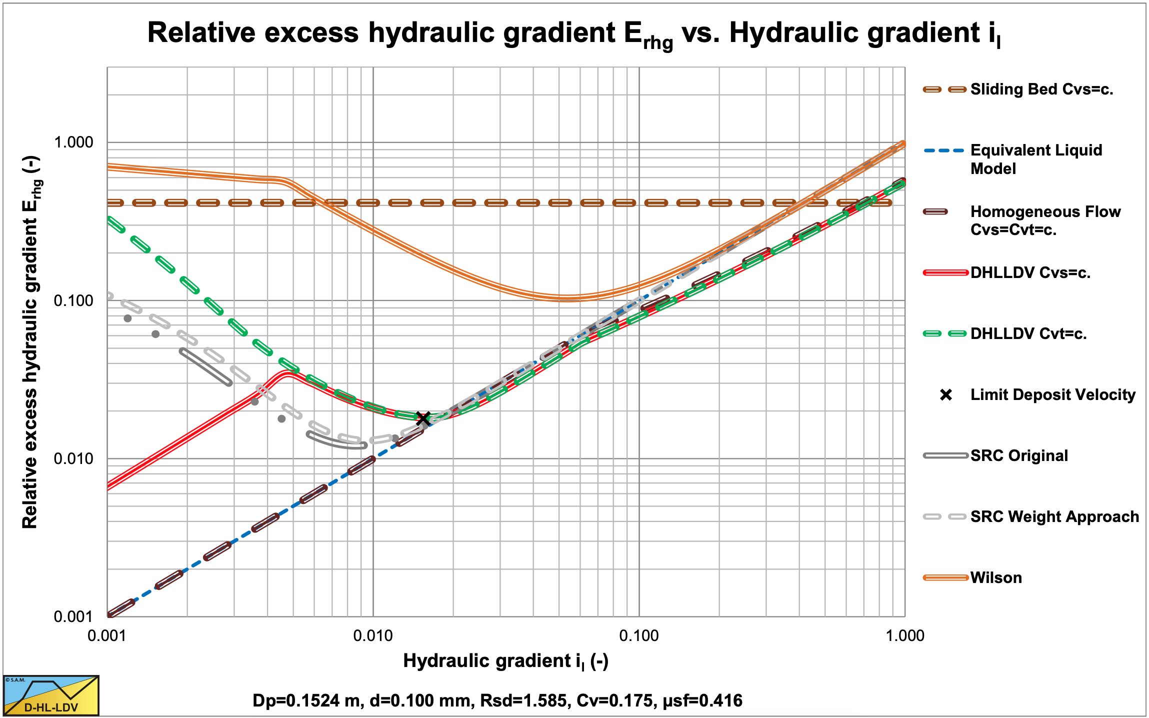
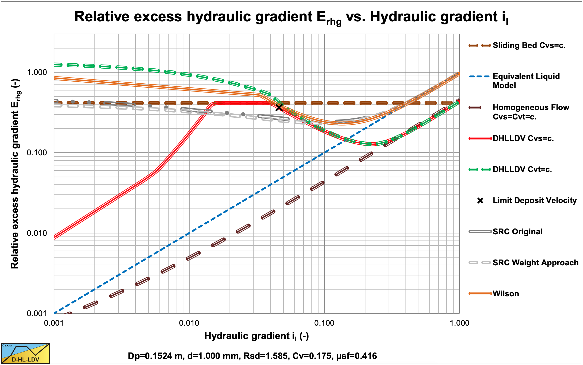
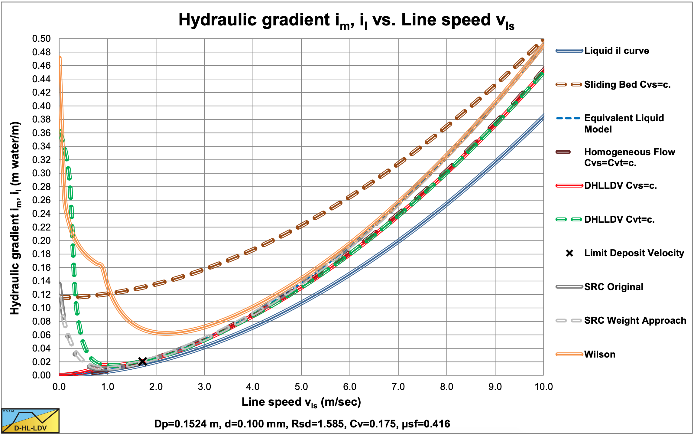
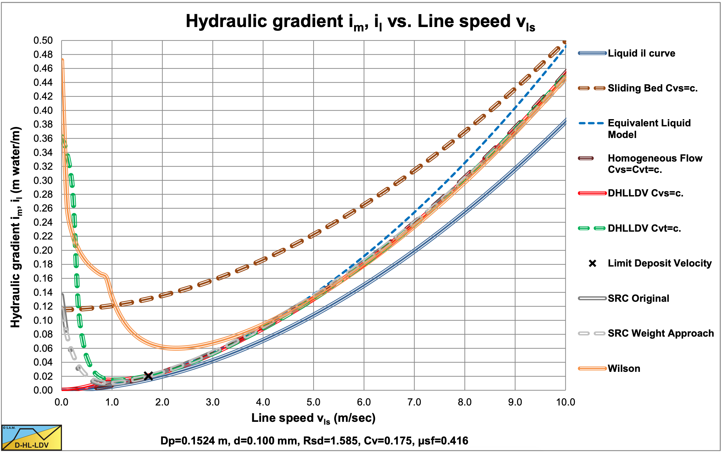
Comparing the SRC model with the DHLLDV Framework and the Wilson et al. (2006) model (equation (6.20-122) and A=1) in a small diameter pipe shows a good resemblance between SRC and DHLLDV for very small particles (Figure 6.22-2) and a good resemblance for coarse particles (Figure 6.22-3) at operational line speeds (il=0.03- 0.1). Both models use constant spatial volumetric concentration, but the SRC model as applied here does not have the stationary bed at low line speeds.
The original SRC model does not show the relative excess hydraulic gradient going below the ELM line, which the DHLLDV Framework does. The behavior of the SRC model for coarse sands looks more like graded sand behavior because the curve is less steep, while the DHLLDV Framework is determined for a uniform sand.
The Wilson et al. (2006) is also shown in the figures. For very small particles this model gives very high values, but for coarser particles is matches very well. This results from the way the v50 is determined. Using a v50 proportional to the terminal settling velocity vt could solve this.
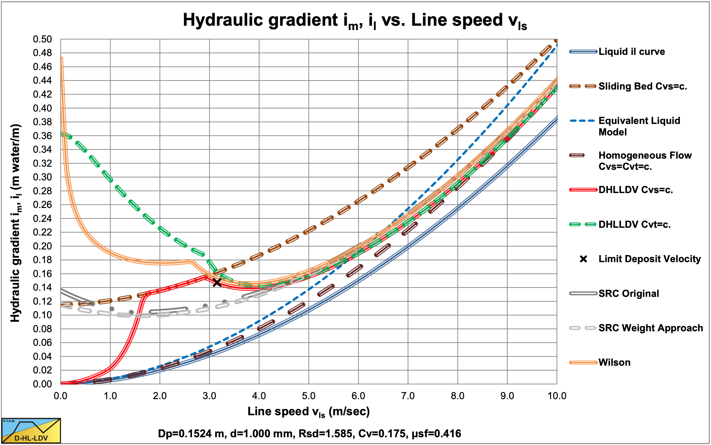
Figure 6.22-4 and Figure 6.22-5 show a comparison for a large diameter pipe. The results are similar to the small diameter pipe. In the line speed region of normal operations, here 5-6 m/sec, the SRC model and the DHLLDV Framework are close. The Wilson et al. (2006) model overestimates the hydraulic gradient for small particles, but matches very well for medium and coarse particles.
The simplification of the SRC model, by using the weight approach of Miedema & Ramsdell (2014) for the sliding friction, shows a very good resemblance in all cases, fine or coarse particles and small or large pipe diameters, although the hydraulic gradient curves found are a bit higher compared with the original SRC model. Only at very low line speeds and high concentrations the two approaches differ, however this is far outside the line speed region of normal operations. As long as the same equation is used for the determination of the contact load fraction, there is not much difference.
It is remarkable that for the Dp=0.762 m (30 inch) pipe and the d=1 mm particle the 3 models give almost the same hydraulic gradient at the LDV.
6.22.8 Further Development of the Model
Experimental evidence of Gillies & Shook (2000A) suggests that an increment in kinetic friction, due to an increase in kinematic particle wall friction, occurs at high concentrations. High means solids concentrations exceeding 30%-35%. A parameter which is useful in quantifying this effect is the linear concentration λlc, which can be considered to be a measure of the ratio of the particle diameter to the shortest distance between neighboring particles:
\[\ \lambda_{\mathrm{lc}}=\frac{1}{\left(\left(\frac{\mathrm{C}_{\mathrm{v b}, \max }}{\mathrm{C}_{\mathrm{v s}}}\right)^{1 / 3}-\mathrm{1}\right)}\]
It is peculiar that in some of the SRC related papers, the term in the denominator is reversed, giving a negative linear concentration. Because this is used squared it has no effect. The above equation is the correct equation (Gillies R. G., 2015). If the liquid density is considered to be appropriate to describe the frictional losses, the frictional losses between the liquid and the pipe wall can be determined with:
\[\ \begin{array}{left} \tau_{1,\mathrm{l}}=\frac{\left(\lambda_{1}+\Delta \lambda_{1}\right)}{4} \cdot \frac{1}{2} \cdot \rho_{\mathrm{l}} \cdot v_{1}^{2}\\\text{With: }\quad \Delta \lambda_{1}=\left(0.0118 \cdot \lambda_{\mathrm{l} \mathrm{c}}\right)^{2}\end{array}\]
At high velocities, when the flow is axially symmetric and Coulomb friction is negligible, the total wall shear stress is regarded as the sum of two contributions. The first contribution is based on the Darcy Weisbach friction factor and the liquid density, the second contribution upon the solids density and the linear concentration. If the friction increment is due to particle wall interactions at high solids concentrations, the total frictional losses between the liquid+particles and the pipe wall can be determined with:
\[\ \begin{array}{left} \tau_{1,\mathrm{l}}=\frac{\left(\lambda_{1} \cdot \rho_{\mathrm{l}}+\lambda_{\mathrm{s}} \cdot \rho_{\mathrm{s}}\right)}{4} \cdot \frac{1}{2} \cdot \mathrm{v}_{1}^{2}\\
\text{With: }\quad \lambda_{\mathrm{s}}=\left(0.0089 \cdot \lambda_{\mathrm{lc}}\right)^{2}\end{array}\]
And:
\[\ \tau_{2,\mathrm{l}}=\frac{\left(\lambda_{1} \cdot \rho_{\mathrm{l}}+\lambda_{\mathrm{s}} \cdot \rho_{\mathrm{s}}\right)}{4} \cdot \frac{1}{2} \cdot \mathrm{v}_{2}^{2}\]
Gillies & Shook (2000A) also presented a slightly different equation for the determination of the contact load fraction:
\[\ \mathrm{\frac{C_{v s, c}}{C_{v s}}=e^{-0.0212 \cdot \frac{v_{l s}}{v_{t}}}}\]
For slurry Reynolds numbers less than 192000 they use:
\[\ \frac{\mathrm{C}_{\mathrm{v s}, \mathrm{c}}}{\mathrm{C}_{\mathrm{v s}}}=\mathrm{e}^{-\mathrm{0 . 0 0 1 0 1 3} \cdot \frac{\mathrm{v}_{\mathrm{l s}}}{\mathrm{v}_{\mathrm{t}}} \cdot \mathrm{R e}^{1 / 4}}\]
This suggests that with highly concentrated slurries of coarse particles, the Coulombic friction increases at low slurry Reynolds numbers.
Later Gillies et al. (2004) give some modifications of the solids term in equation (6.22-41) related to high line speeds. Assuming the Coulombic friction is negligible compared to the kinematic friction, the solids Darcy Weisbach friction coefficient is modified to:
\[\ \begin{array}{left} \lambda_{\mathrm{s}}=4 \cdot \lambda_{\mathrm{lc}}^{1.25} \cdot\left(0.00005+0.00033 \cdot \mathrm{e}^{-0.1 \cdot \mathrm{d}^{+}}\right)\\
\text{With : }\quad \mathrm{d}^{+}=\frac{\mathrm{d} \cdot \mathrm{u}_{*}}{v_{\mathrm{l}}}=\frac{\mathrm{d} \cdot \sqrt{\frac{\lambda_{\mathrm{l}}}{\mathrm{8}}}{ \cdot \mathrm{v}_{\mathrm{ls}}}}{v_{\mathrm{l}}}\end{array}\]
Although this correlation was obtained at high line speeds, where the effect of Coulombic friction is small, indications show that it is applicable to kinematic friction at all line speeds. A change in the method of predicting the kinematic friction, forces the correlation that is used for predicting the contact load fraction to be modified. Apparently this contact load fraction is a virtual contact load fraction depending on the other parts of the SRC model. The equation for the contact load fraction is now modified to:
\[\ \begin{array}{left}\frac{\mathrm{C}_{\mathrm{v s}, \mathrm{c}}}{\mathrm{C}_{\mathrm{v s}}}&=\mathrm{e}^{-\mathrm{0 . 0 0 9 7} \cdot\left(\frac{\mathrm{v}_{\mathrm{ls}}}{\mathrm{v}_{\mathrm{t}}}\right)^{0.864} \cdot \mathrm{R e}^{0.193} \cdot \mathrm{F r}^{-0.292}}\\
\operatorname{Re}&=\frac{\mathrm{D}_{\mathrm{p}} \cdot \mathrm{v}_{\mathrm{l s}}}{v_{\mathrm{l}}} \cdot \frac{1}{1+\mathrm{0 . 2 1} \cdot \lambda_{\mathrm{m}}^{2}} \quad\text { or 120000, whichever is less}\\
\mathrm{F r}&=\frac{\mathrm{v}_{\mathrm{l s}}}{\left(\mathrm{g} \cdot \mathrm{D}_{\mathrm{p}} \cdot \mathrm{R}_{\mathrm{s d}}\right)} \quad\text{
or 3.0, whichever is less} \end{array}\]
The sliding friction factor (Coulombic friction) depends on the ratio of the thickness of the viscous sub layer to the particle diameter, with μsf0=0.5, according to:
\[\ \begin{array}{left} \mu_{\mathrm{sf}}=\mu_{\mathrm{sf} 0} \cdot\left(2 \cdot\left(1-\frac{\delta_{\mathrm{v}}}{\mathrm{d}}\right)\right)\\
\text{With : }\quad \delta_{\mathrm{v}}=5 \cdot \frac{v_{\mathrm{l}}}{\mathrm{u}_{*}}\\
\text{With : }\quad 0.1 \leq\left(2 \cdot\left(1-\frac{\delta_{\mathrm{v}}}{\mathrm{d}}\right)\right) \leq 1\end{array}\]
This is of course an adjustment only important for very small particles. SRC found that this adjustment is important for the industrial slurries that were tested at the SRC Pipe Flow Technology Centre. Depending on factors such as the viscosity of the carrier fluid (water and clays), particles with diameters as large as 0.2 mm may contribute significantly to the total kinematic friction (i.e. λs is significantly greater than zero). The vast majority of the industrial slurries contain significant concentrations of particles that are 0.2 mm or less (Gillies R. G., 2015). D.P. Gillies (2013) adjusted the equation for the Darcy Weisbach solids contribution friction factor to:
\[\ \begin{array}{left}&\lambda_{\mathrm{s}}=4 \cdot \lambda_{\mathrm{lc}} ^ {1.25} \cdot\left(\mathrm{A} \cdot \ln \left(\mathrm{d}^{+}\right)+\mathrm{B}\right)\\
\text{With: }&\mathrm{A}=-\mathrm{0 . 0 0 0 1 1 0}\quad\text{ and }\quad\mathrm{B}=\mathrm{0 . 0 0 0 4 2}\quad\text{ for }\quad\mathrm{d}^{+} \leq \mathrm{1 9 . 3 6}\\
&\mathrm{A}=-\mathrm{0 . 0 0 0 0 5 6} \quad\text { and }\quad \mathrm{B}=\mathrm{0 . 0 0 0 2 6} \quad\text { for }\quad \mathrm{d}^{+}>\mathrm{1 9 . 3 6} \\
&\mathrm{A}=\mathrm{0} \quad \text { and } \quad \mathrm{B}=\mathrm{0}\quad\text{ for }\quad \mathrm{d}^{+}>\mathrm{1 0 3 . 8 4}\end{array}\]
6.22.9 Final Conclusions
The model uses spatial concentration in its inner workings and it predicts delivered concentrations. If the delivered concentration is specified, then iteration is required to come up with the spatial concentration that offers the specified delivered concentration. A model is developed at SRC to predict the concentration distribution. This model’s prediction is used to set the concentration in the lower layer of the two-layer model. The latest version of the SRC model can be summarized with the following equations:
The Erhg value is the excess hydraulic gradient im-il divided by the relative submerged density Rsd and the spatial volumetric concentration Cvs.
\[\ \mathrm{E_{rhg}=\frac{i_m - i_l}{C_{vs}\cdot R_{sd}}}=\frac{ \left(\begin{array}{l}\mu_{\mathrm{sf}} \cdot \mathrm{C}_{\mathrm{vs}, 2} \cdot \frac{2 \cdot(\sin (\beta)-\beta \cdot \cos (\beta))}{\pi} \cdot \frac{\left(1-\mathrm{C}_{\mathrm{vs}, 1}-\mathrm{C}_{\mathrm{vs}, 2}\right)}{\left(1-\mathrm{C}_{\mathrm{vs}, 2}\right)} \\ +\lambda_{\mathrm{s}} \cdot \frac{\rho_{\mathrm{s}}}{\rho_{\mathrm{l}}} \cdot \frac{1}{2 \cdot \mathrm{g} \cdot \mathrm{D}_{\mathrm{p}} \cdot \mathrm{R}_{\mathrm{sd}}} \cdot \mathrm{v_{\mathrm{ls}}}^{2}\end{array}\right)}{\mathrm{C_{vs}}}\]
In terms of the weight approach the following can be derived:
\[\ \mathrm{E}_{\mathrm{rhg}}=\frac{\left(\mu_{\mathrm{sf}} \cdot \mathrm{C}_{\mathrm{vs}, \mathrm{c}}+\lambda_{\mathrm{s}} \cdot \frac{\rho_{\mathrm{s}}}{\rho_{\mathrm{l}}} \frac{1}{2 \cdot \mathrm{g} \cdot \mathrm{D}_{\mathrm{p}} \cdot \mathrm{R}_{\mathrm{sd}}} \cdot \mathrm{v}_{\mathrm{ls}}^{2}\right)}{\mathrm{C}_{\mathrm{vs}}}\]
At very low line speeds, the contact load concentration Cvs,c=Cvs and the equations reduce to:
\[\ \mathrm{E}_{\mathrm{rhg}}=\frac{\mathrm{i}_{\mathrm{m}}-\mathrm{i}_{\mathrm{l}}}{\mathrm{C}_{\mathrm{v} \mathrm{s}} \cdot \mathrm{R}_{\mathrm{s} \mathrm{d}}}=\mu_{\mathrm{sf}} \cdot \frac{2 \cdot(\sin (\beta)-\beta \cdot \cos (\beta))}{\pi}\]
Which is the 2LM solution of Wilson (2006). In terms of the weight approach the following can be derived:
\[\ \mathrm{E}_{\mathrm{r h g}}=\mu_{\mathrm{s f}}\]
Which is the sliding bed equation according to Miedema & Ramsdell (2014).
At very high line speeds, the contact load concentration Cvs,c=0 and the equations reduce to:
\[\ \mathrm{E}_{\mathrm{r h g}}=\frac{\lambda_{\mathrm{s}} \cdot \rho_{\mathrm{s}} \cdot \frac{\mathrm{1}}{2} \cdot \mathrm{v}_{\mathrm{l} s}^{2}}{\rho_{\mathrm{l}} \cdot \mathrm{g} \cdot \mathrm{D}_{\mathrm{p}} \cdot \mathrm{R}_{\mathrm{s d}} \cdot \mathrm{C}_{\mathrm{v s}}}=\frac{\lambda_{\mathrm{s}} \cdot \rho_{\mathrm{s}}}{\lambda_{\mathrm{l}} \cdot \rho_{\mathrm{l}}} \cdot \frac{\mathrm{1}}{\mathrm{R}_{\mathrm{s d}} \cdot \mathrm{C}_{\mathrm{v s}}} \cdot \frac{\lambda_{\mathrm{l}} \cdot \mathrm{v}_{\mathrm{l s}}^{2}}{\mathrm{2} \cdot \mathrm{g} \cdot \mathrm{D}_{\mathrm{p}}}=\frac{\lambda_{\mathrm{s}} \cdot \mathrm{\rho}_{\mathrm{s}}}{\lambda_{\mathrm{l}} \cdot \mathrm{\rho}_{\mathrm{l}}} \cdot \frac{\mathrm{1}}{\mathrm{R}_{\mathrm{s d}} \cdot \mathrm{C}_{\mathrm{v s}}} \cdot \mathrm{i}_{\mathrm{l}}\]
The kinetic friction factor contains \(\ \lambda_{\mathrm{lc}}^{1.25}\), which depends on the relative concentration Cvr=Cvs/Cvb. This gives:
\[\ \lambda_{\mathrm{lc}}=\frac{\mathrm{C}_{\mathrm{vr}}^{1 / 3}}{\left(1-\mathrm{C}_{\mathrm{vr}}^{1 / 3}\right)}\]
This gives:
\[\ \mathrm{E}_{\mathrm{rhg}}=4 \cdot\left(\frac{\mathrm{C}_{\mathrm{vr}}^{1 / 3}}{\left(1-\mathrm{C}_{\mathrm{vr}}^{1 / 3}\right)}\right)^{1.25} \cdot \frac{\left(0.00005+0.00033 \cdot \mathrm{e}^{-0.1 \cdot \mathrm{d}^{+}}\right)}{\lambda_{\mathrm{l}} \cdot \mathrm{R}_{\mathrm{sd}} \cdot \mathrm{C}_{\mathrm{vb}} \cdot \mathrm{C}_{\mathrm{vr}}} \cdot \frac{\rho_{\mathrm{s}}}{\rho_{\mathrm{l}}} \cdot \mathrm{i}_{\mathrm{l}}\]
Or:
\[\ \mathrm{E}_{\mathrm{rhg}}=4 \cdot\left(\frac{\mathrm{C}_{\mathrm{vr}}^{1 / 3}}{\left(1-\mathrm{C}_{\mathrm{vr}}^{1 / 3}\right)}\right)^{1.25} \cdot \frac{\left(\mathrm{A} \cdot \ln \left(\mathrm{d}^{+}\right)+\mathrm{B}\right)}{\lambda_{\mathrm{l}} \cdot \mathrm{R}_{\mathrm{sd}} \cdot \mathrm{C}_{\mathrm{vb}} \cdot \mathrm{C}_{\mathrm{vr}}} \cdot \frac{\rho_{\mathrm{s}}}{\rho_{\mathrm{l}}} \cdot \mathrm{i}_{\mathrm{l}}\]
Using the ELM for any line speed gives:
\[\ \mathrm{E}_{\mathrm{r h g}}=\mathrm{i}_{\mathrm{l}}\]
So the factor in front of the liquid hydraulic gradient is a sort of multiplication factor related to the ELM. Equation (6.22-55) gives a multiplication factor according to Figure 6.22-6 (determined with λl=0.015) for different values of the dimensionless particle diameter. For normal relative concentrations at very high line speeds this factor is about 0.35, meaning that about 35% of the solids effect of the ELM will be taken into account. For very low and high relative concentrations the multiplication factor is greater than 1, which seems too high, since it implies a solids effect greater than the solids effect of the ELM. This also occurs for values of the dimensionless particle diameter at below 100. Equation (6.22-57) gives a multiplication factor of zero for dimensionless particles diameters above 100, meaning that there is no solids effect, just pure liquid resistance.
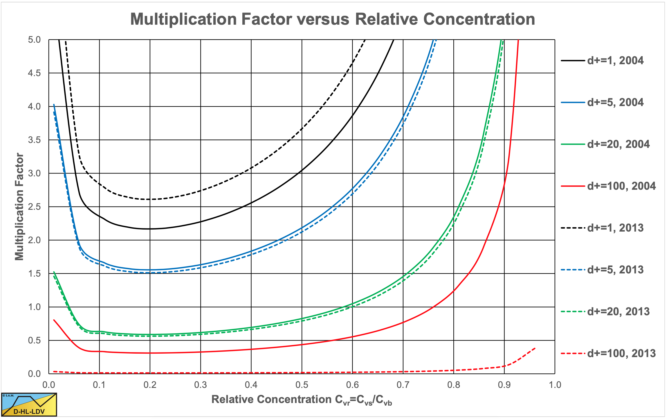
Equation (6.22-57) gives a multiplication factor of zero for very high line speeds, resulting in a solids effect of zero. This means that at very high line speeds the resistance or hydraulic gradient equals the pure liquid resistance or hydraulic gradient.
Whether the head losses approach the pure liquid head losses it very high line speeds is the question. The concept that solids do not have any effect anymore, even at high concentrations is difficult to defend. Unfortunately there are no experimental data for such high line speeds. The data available show that at high line speeds the head losses are somewhere between the ELM and the pure liquid head losses. A factor of 0.6 or 60% of the solids effect seems reasonable.
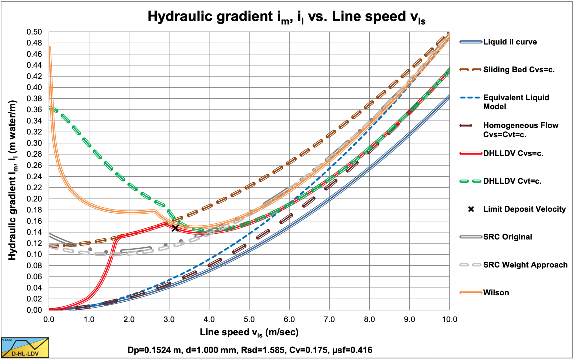
Figure 6.22-7 and Figure 6.22-8 show the comparison between the 2004 SRC model, the DHLLDV Framework and the Wilson et al. (2006) model (equation (6.20-122) and A=0.6) for a Dp=0.1524 m (6 inch) pipe and particles with d=0.1 mm and d=1 mm. For the d=0.1 mm particle, SRC and DHLLDV match again very well for Erhg=0.03- 0.1. Wilson et al. (2006) overestimates as discussed before. For the d=1 mm particle the 3 models match very well for Erhg=0.03-0.1. The SRC model and the Wilson et al. (2006) model curves are a bit lower compared with Figure 6.22-2 and Figure 6.22-3 giving a better correlation with the DHLLDV Framework.
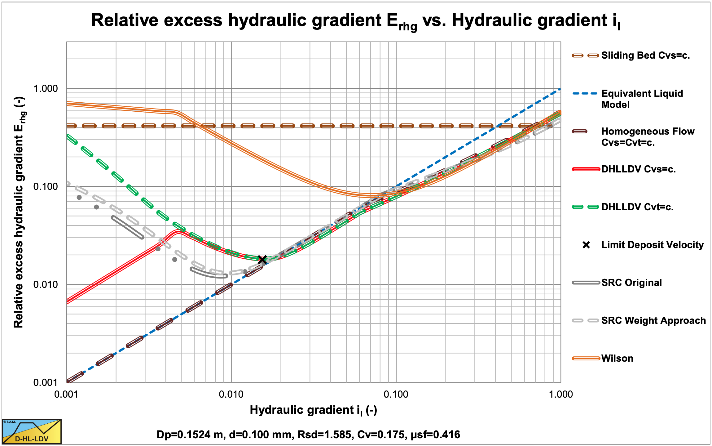
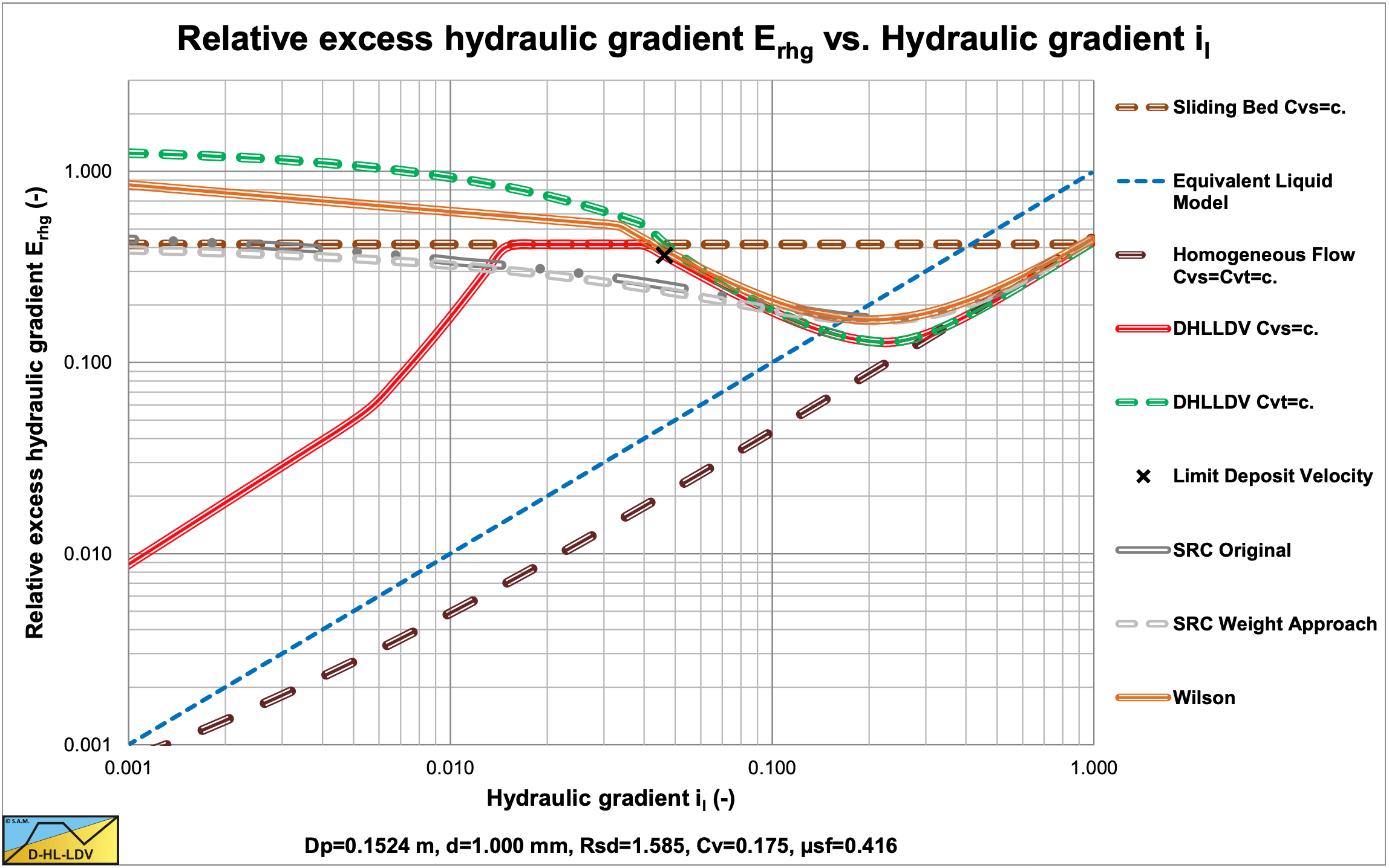
Figure 6.22-9 and Figure 6.22-10 show the comparison between the 2004 SRC model, the DHLLDV Framework and the Wilson et al. (2006) model (equation (6.20-122) and A=0.6) for a Dp=0.762 m (30 inch) pipe and particles with d=0.1 mm and d=1 mm. For the d=0.1 mm particle, SRC and DHLLDV match again very well for line speeds between 4 and 7 m/s. Wilson et al. (2006) overestimates as discussed before. For the d=1 mm particle the 3 models match very well for line speeds between 4 and 7 m/s.
6.22.10 The Limit Deposit Velocity
Gillies (1993) derived an expression for the Durand & Condolios (1952) Froude number FL, giving a Limit Deposit Velocity of:
\[\ \mathrm{v}_{\mathrm{l s}, \mathrm{l d v}}=\mathrm{e}^{\left(\mathrm{0 . 5 1 - 0 . 0 0 7 3 . C _ { \mathrm { D } } - \mathrm { 1 2 . 5 }} \cdot\left(\frac{(\mathrm{g}{ \cdot v _ { \mathrm{l} }})^{2 / 3}}{\mathrm{g \cdot d}}-\mathrm{0 . 1 4}\right)^{2}\right)} \cdot \sqrt{\mathrm{2 \cdot \mathrm { g } \cdot \mathrm { D } _ { \mathrm { p } } \cdot \mathrm { R } _ { \mathrm { s d } }}}\]
With the Froude number FL:
\[\ \mathrm{F}_{\mathrm{L}}=\frac{\mathrm{v}_{\mathrm{l s}, \mathrm{ld v}}}{\sqrt{\mathrm{2} \cdot \mathrm{g} \cdot \mathrm{D}_{\mathrm{p}} \cdot \mathrm{R}_{\mathrm{s d}}}}=\mathrm{e}^{\left(\mathrm{0 . 5 1 - 0 . 0 0 7 3 .} \mathrm{C}_{\mathrm{D}}-\mathrm{1 2 . 5} \cdot\left(\frac{\left(\mathrm{g} \cdot v_{\mathrm{l}}\right)^{2 / 3}}{\mathrm{g} \cdot \mathrm{d}}-\mathrm{0 . 1 4}\right)^{2}\right)}\]
The Durand & Condolios (1952) Froude number FL does not depend on the pipe diameter and the volumetric concentration. The Froude number FL should be considered the maximum FL at a concentration near 20%. The FL value increases with the particle diameter to a maximum of 1.64 for d=0.4 mm after which it decreases slowly to an asymptotic value of about 1.3 for very large particles. This is consistent with Wilson’s (1979) nomogram (which gives the LSDV) and consistent with the FL graph published by Durand & Condolios (1952). Quantitatively this equation matches the graph of Durand (1953), which differs by a factor 1.28 (to high) from the original graph of Durand & Condolios (1952).
Shook et al. (2002) give the following correlations for the Durand Froude number FL:
\[\ \begin{array}{left} \mathrm{F_{\mathrm{L}}}=\frac{\mathrm{v}_{\mathrm{ls}, \mathrm{ldv}}}{\sqrt{2 \cdot \mathrm{g} \cdot \mathrm{D}_{\mathrm{p}} \cdot \mathrm{R}_{\mathrm{sd}}}}=0.197 \cdot \operatorname{Ar}^{0.4}=0.197 \cdot\left(\frac{4 \cdot \mathrm{g} \cdot \mathrm{d}^{3} \cdot \mathrm{R}_{\mathrm{sd}}}{3 \cdot v_{\mathrm{l}}^{2}}\right)^{0.4}\quad\text{ for }\quad80<\mathrm{Ar}<160\\
\mathrm{F}_{\mathrm{L}}=\frac{\mathrm{v}_{\mathrm{ls}, \mathrm{ldv}}}{\sqrt{2 \cdot \mathrm{g} \cdot \mathrm{D}_{\mathrm{p}} \cdot \mathrm{R}_{\mathrm{sd}}}}=1.19 \cdot \mathrm{Ar}^{0.045}=1.19 \cdot\left(\frac{4 \cdot \mathrm{g} \cdot \mathrm{d}^{3} \cdot \mathrm{R}_{\mathrm{sd}}}{3 \cdot v_{\mathrm{l}}^{2}}\right)^{0.045}\quad\text{ for }\quad160<\mathrm{Ar}<540\\
\mathrm{F}_{\mathrm{L}}=\frac{\mathrm{v}_{\mathrm{ls}, \mathrm{ldv}}}{\sqrt{2 \cdot \mathrm{g} \cdot \mathrm{D}_{\mathrm{p}} \cdot \mathrm{R}_{\mathrm{sd}}}}=1.78 \cdot \mathrm{Ar}^{-0.019}=1.78 \cdot\left(\frac{4 \cdot \mathrm{g} \cdot \mathrm{d}^{3} \cdot \mathrm{R}_{\mathrm{sd}}}{3 \cdot v_{\mathrm{l}}^{2}}\right)^{-0.019} \quad \text{for}\quad540<\mathrm{Ar}\end{array}\]
The Durand & Condolios (1952) Froude number FL does not depend on the pipe diameter and the volumetric concentration. The Froude number FL should be considered the maximum FL at a concentration near 20%.
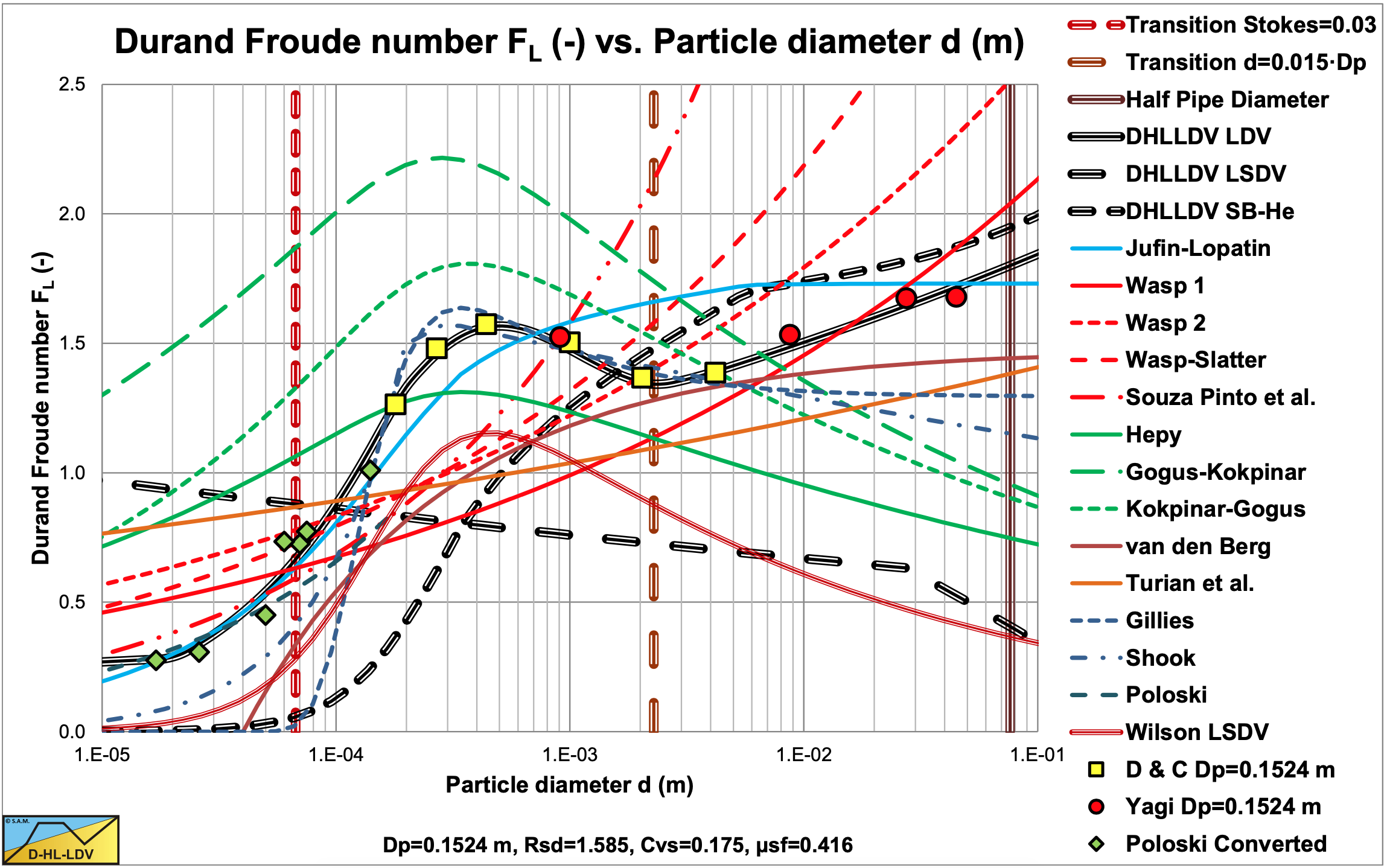
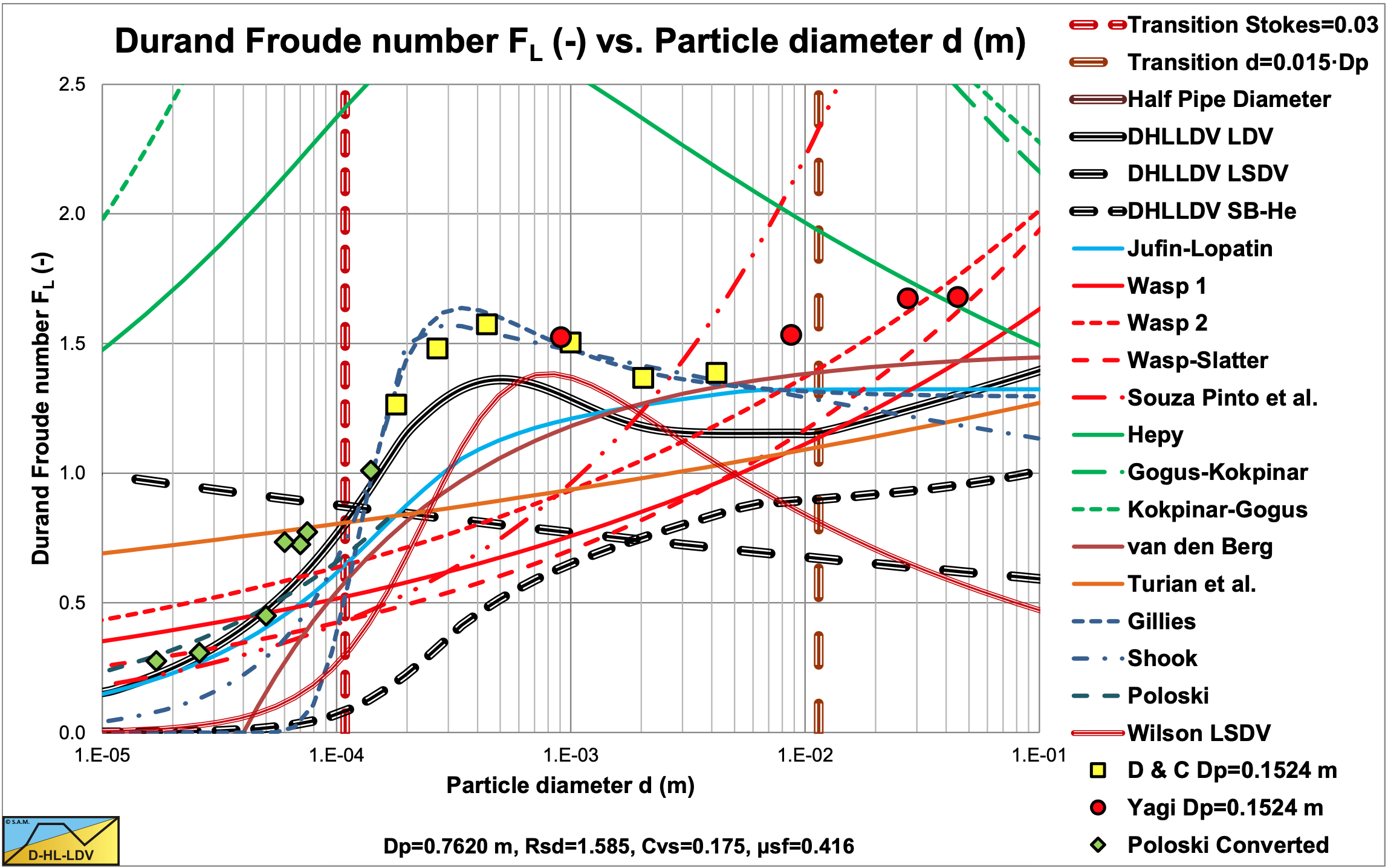
Figure 6.22-11 and Figure 6.22-12 show the Durand & Condolios (1952) Froude number FL for small and large pipe diameters in comparison with many other FL or LDV equations. For small pipe diameters the Gillies (1993) and Shook et al. (2002) equations match well with the DHLLDV Frameworks, but for large pipe diameters they give higher values, since both Gillies (1993) and Shook et al. (2002) have no dependency of the FL number with respect to the pipe diameter, while the DHLLDV Framework has.
Both models seem to be a fit to the Durand (1953) graph, although based on their own data. As will be concluded more often, the wrong Durand (1953) graph seems to be right based on many data of many researchers. The original Durand & Condolios (1952) graph seems to underestimate the Limit Deposit Velocity.
Figure 6.22-13 shows Durand Froude numbers of Gillies et al. (2000B) and others for a 0.1524 m diameter pipe. The Gillies et al. (2000B) values were originally with the Archimedes number on the abscissa and are transferred to particle diameter for the case all data points were for sand/gravel.

6.22.11 Experiments
Gillies (1993) carries out experiments with small and large pipe diameters and with fine and coarse sand. Some of these experiments with large pipe diameters are shown in the following figures. Figure 6.22-15 shows the data points for a d=0.18 mm sand in a Dp=0.495 m diameter pipe. The data points do not really match the theoretical curve based on the DHLLDV Framework. Figure 6.22-16 shows the same data points, but here the Thomas (1965) viscosity is included in the DHLLDV Framework, based on about 50% of the concentration. Now there is a good match between experiments and theory.
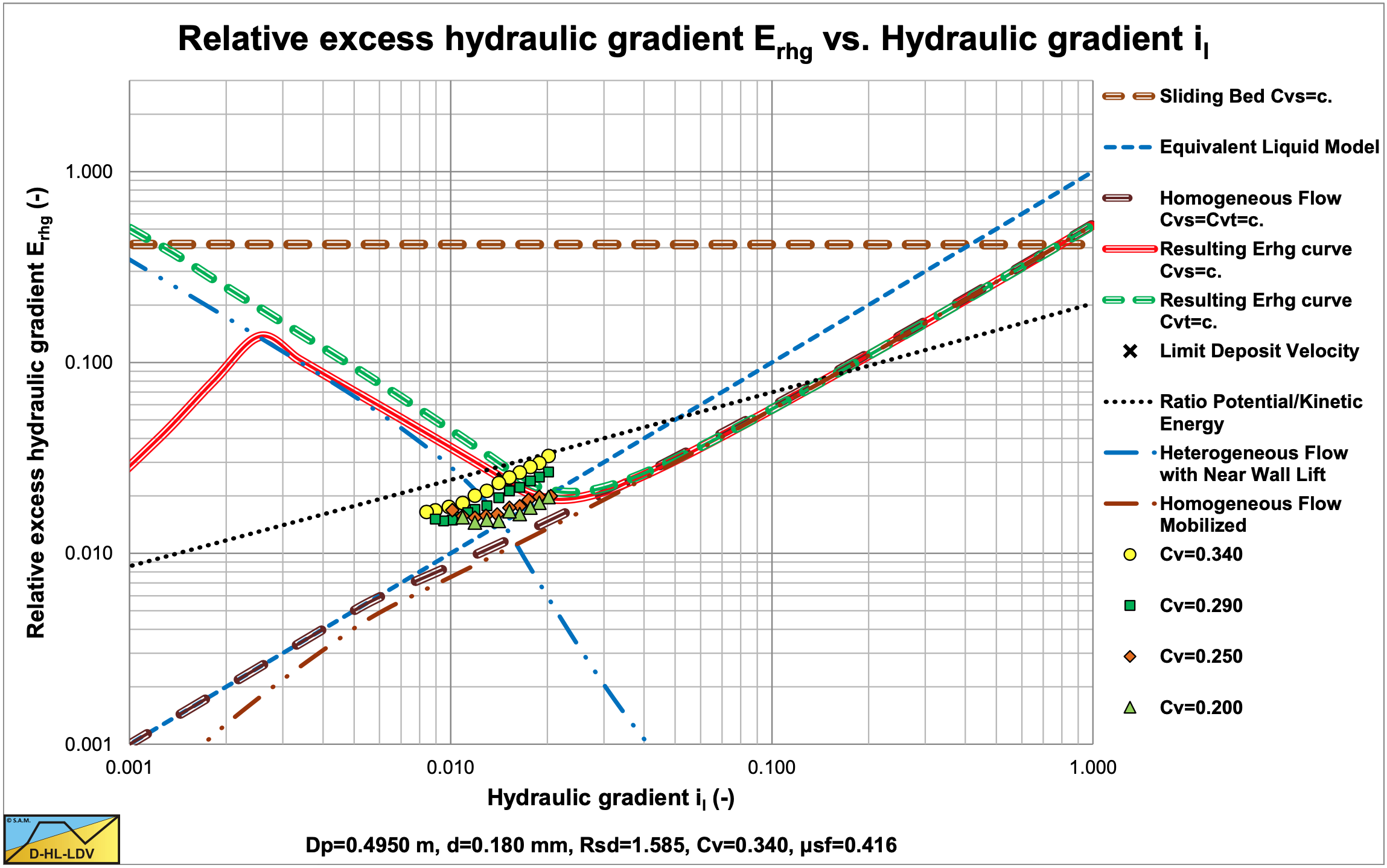
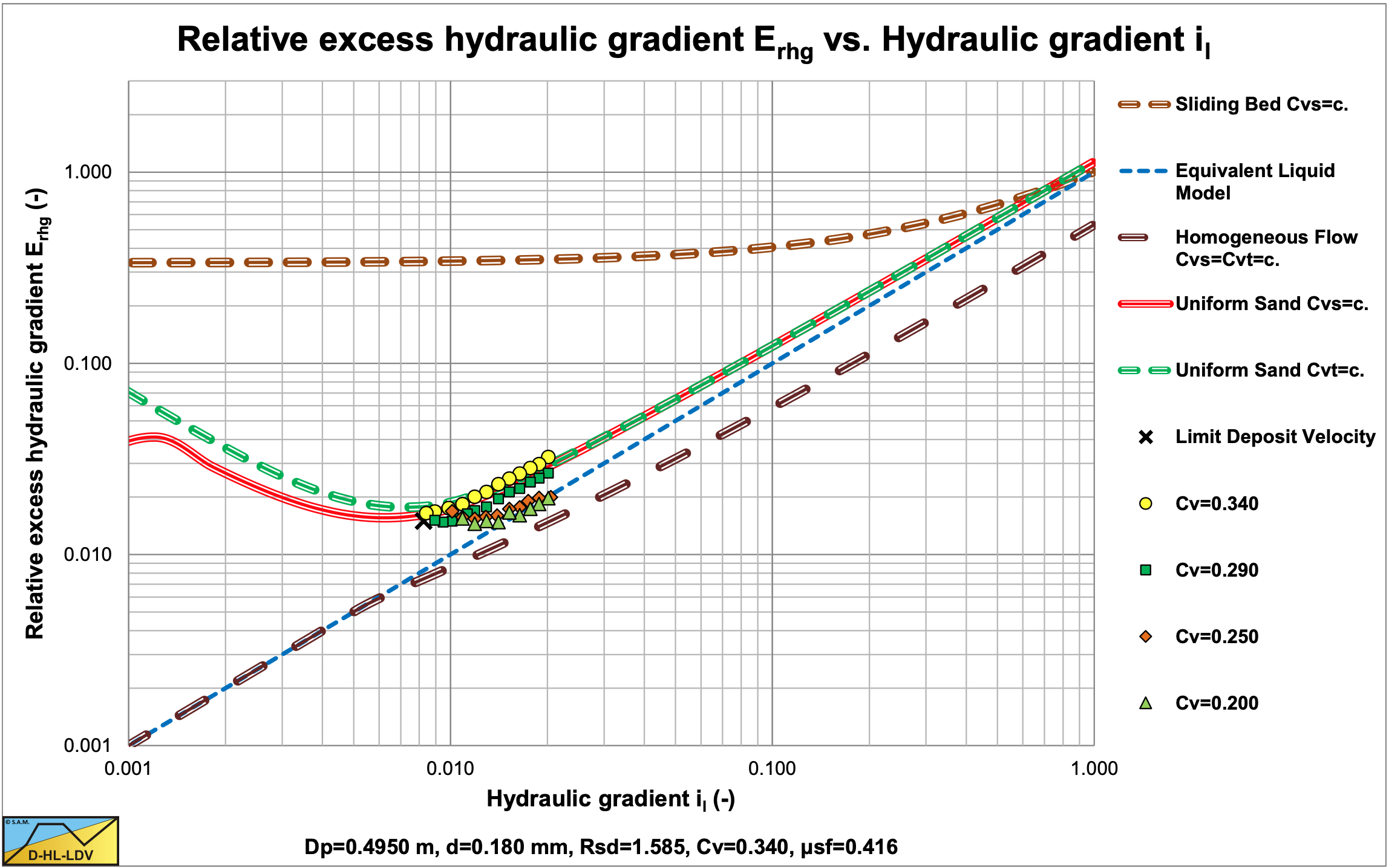
Figure 6.22-17 shows the data points for a d=0.29 mm sand in a Dp=0.263 m diameter pipe. The data points match the theoretical curve based on the DHLLDV Framework reasonably.
Figure 6.22-18 shows the same data points, but here the Thomas (1965) viscosity is included in the DHLLDV Framework, based on about 25% of the concentration. Now there is a good match between experiments and theory.
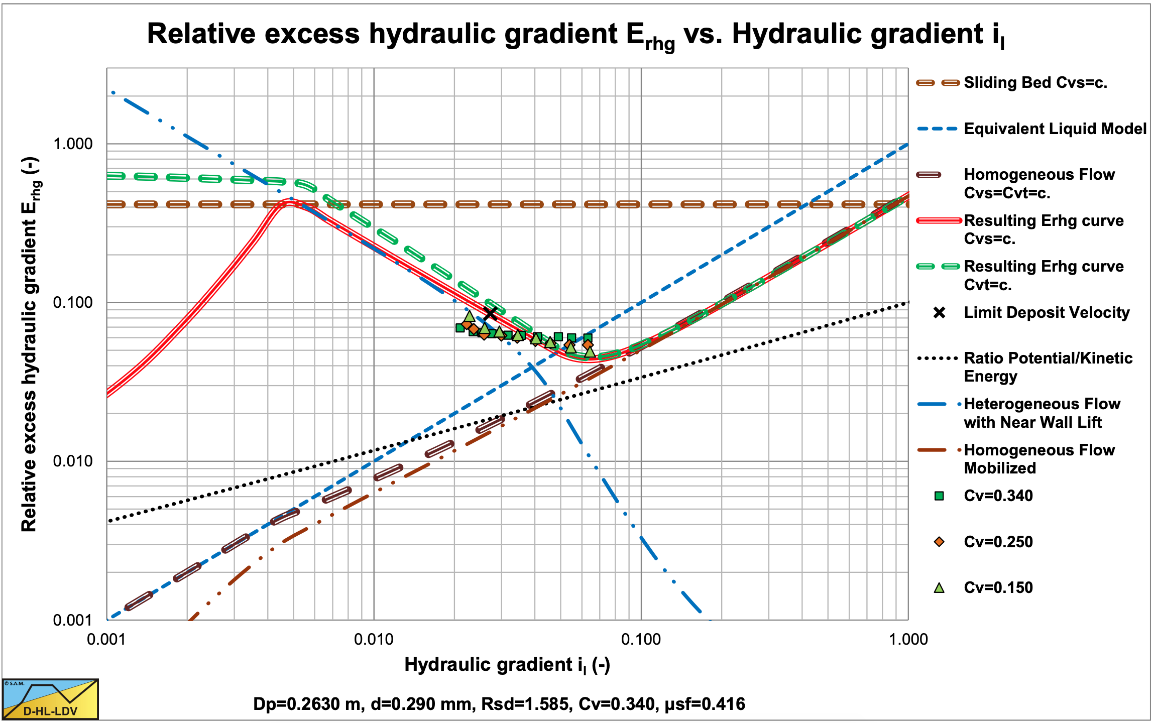
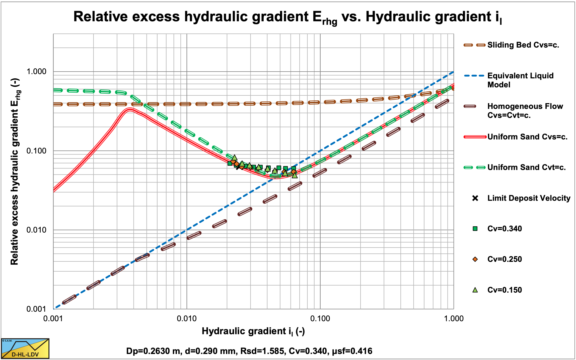
Figure 6.22-19 shows the data points for a d=0.38 mm sand in a Dp=0.263 m diameter pipe. The data points match the theoretical curve based on the DHLLDV Framework reasonably. Figure 6.22-20 shows the same data points, but here the Thomas (1965) viscosity is included in the DHLLDV Framework, based on about 25% of the concentration. Now there is a good match between experiments and theory. Apparently the influence of the Thomas (1965) viscosity reduces if the particles size increases. The influence of the Thomas (1965) viscosity is probably smooth. With 100% for very fine particles, reducing to zero for medium sized particles.
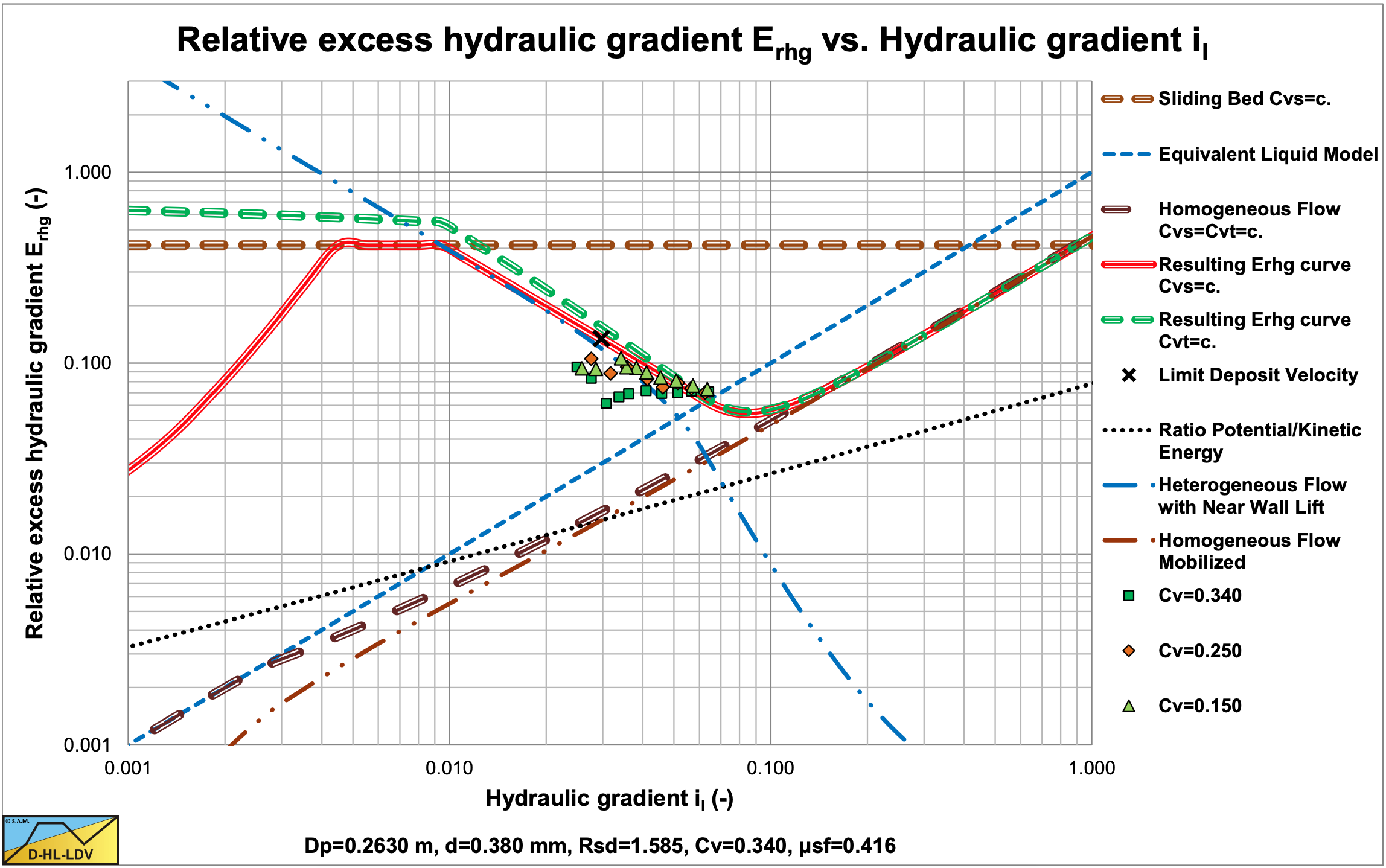
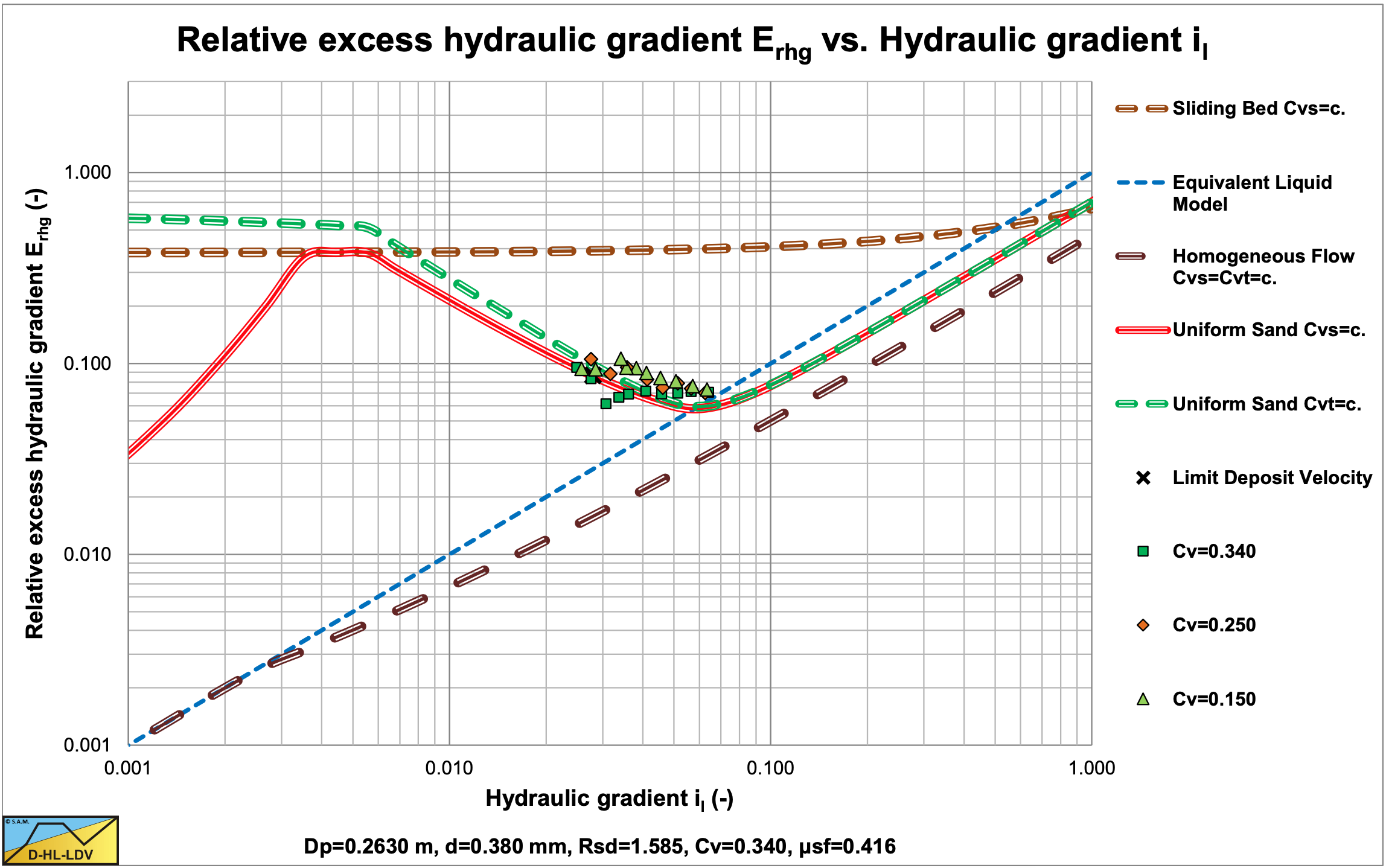
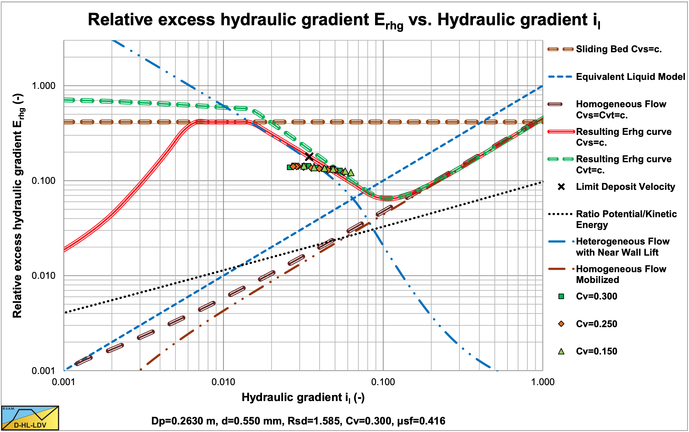
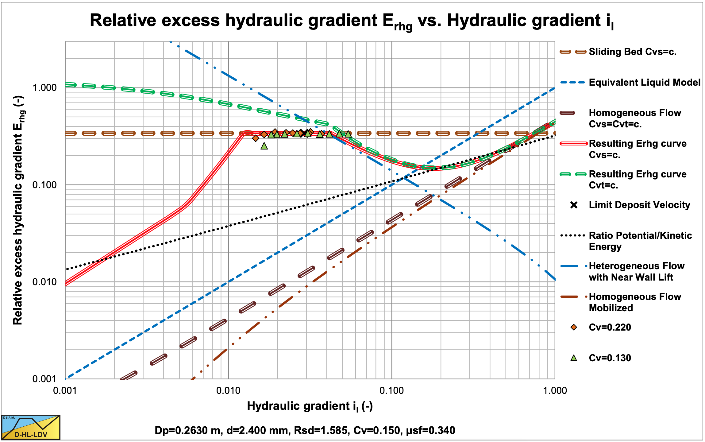
Figure 6.22-21 shows the data points for a d=0.55 mm sand in a Dp=0.263 m diameter pipe. Different concentrations cannot be distinguished, meaning that the hydraulic gradient is proportional to the volumetric concentration. The steepness of the data points is much less than the prediction with the DHLLDV Framework. This may be the result of grading.
Figure 6.22-22 shows the data points for a d=2.4 mm sand in a Dp=0.263 m diameter pipe. Here the data points confirm the existence of a sliding bed and again different concentrations cannot be distinguished.
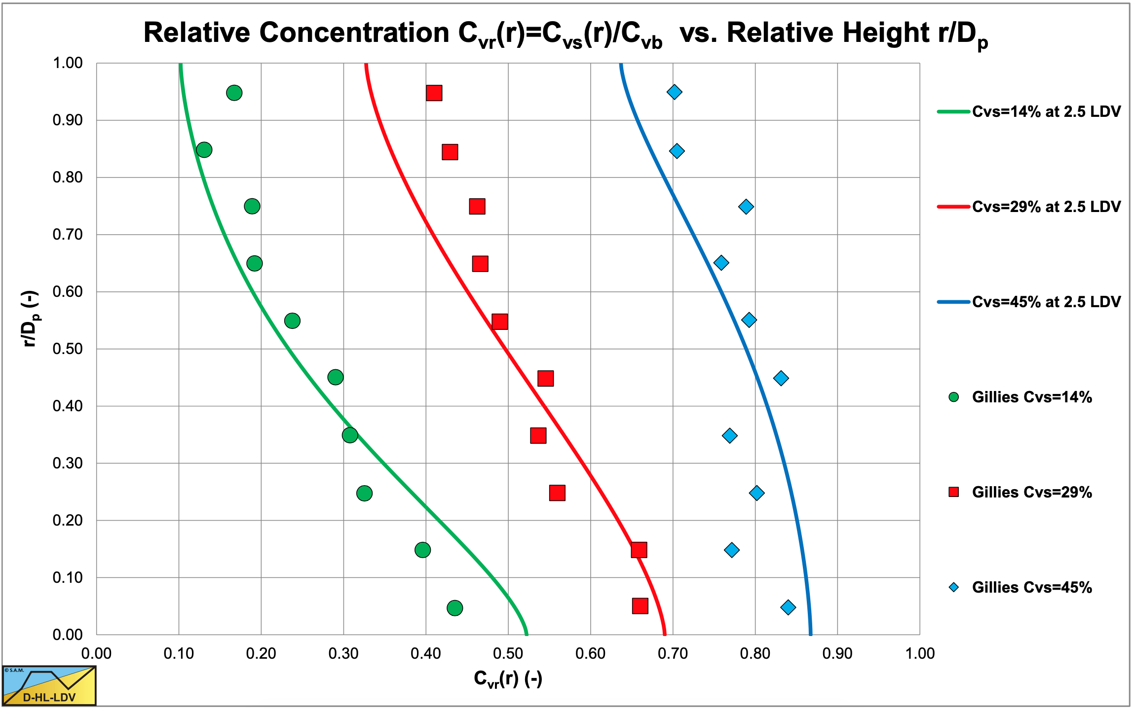
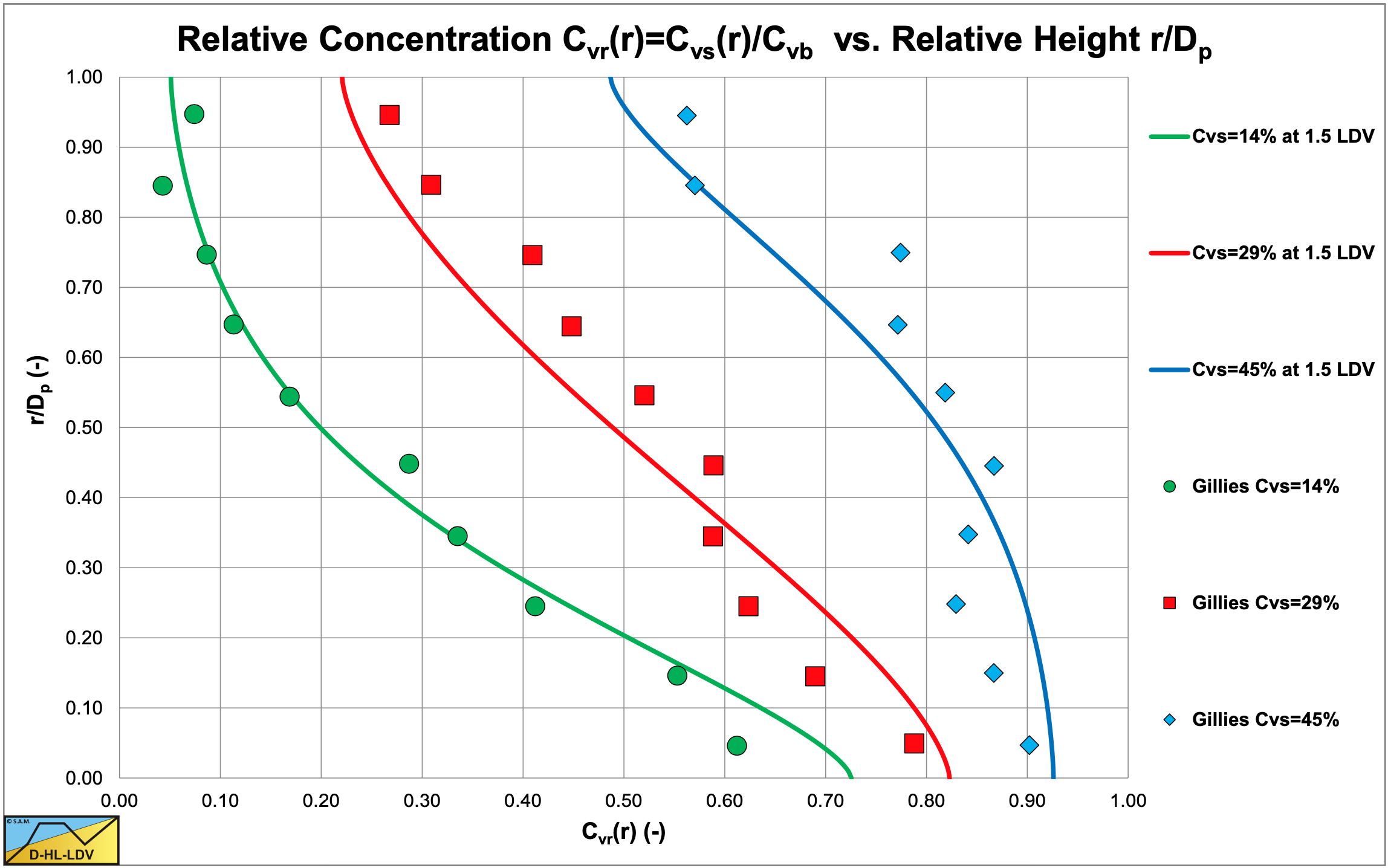
Figure 6.22-23 and Figure 6.22-24 show the concentration distributions for 3 average volumetric concentrations and 2 line speeds for a pipe diameter of Dp=0.0532 m and a particle diameter of d=0.18 m. The LDV (the line speed where there is no bed anymore) is about 1.2 m/s for a 17.5% volumetric concentration and slightly lower for the higher concentrations. The fit lines are based on the DHLLDV Framework, assuming a bed concentration of 55%. So at a line speed of 1.8 m/s a bottom concentration lower than the bed concentration is expected, but at 3.1 m/s a much lower bottom concentration and a slightly steeper concentration profile is expected.
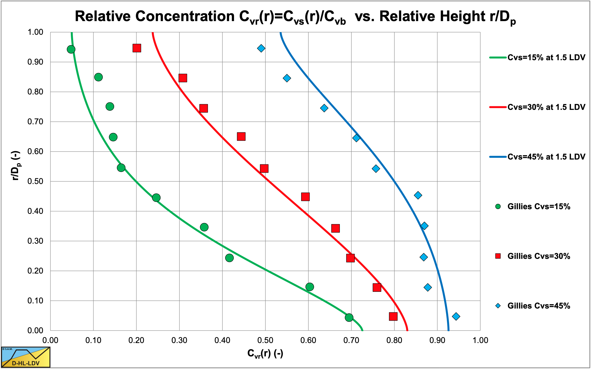
Figure 6.22-25 and Figure 6.22-26 show the concentration distributions for 3 average volumetric concentrations and 2 line speeds for a pipe diameter of Dp=0.0532 m and a particle diameter of d=0.29 m. The LDV (the line speed where there is no bed anymore) is about 1.8 m/s for a 17.5% volumetric concentration and slightly lower for the higher concentrations. The fit lines are based on the DHLLDV Framework, assuming a bed concentration of 55%. So at a line speed of 1.8 m/s a bottom concentration close to the bed concentration is expected, but at 3.1 m/s a lower bottom concentration and a slightly steeper concentration profile is expected.
Figure 6.22-27 and Figure 6.22-28 show the concentration distributions for 3 average volumetric concentrations and 2 line speeds for a pipe diameter of Dp=0.0532 m and a particle diameter of d=0.55 m. The LDV (the line speed where there is no bed anymore) is about 2.2 m/s for a 17.5% volumetric concentration and slightly lower for the higher concentrations. The fit lines are based on the DHLLDV Framework, assuming a bed concentration of 55%. So at a line speed of 2.1 m/s a bottom concentration close to the bed concentration is expected. At 3.1 m/s a slightly lower bottom concentration and a slightly steeper concentration profile is expected.
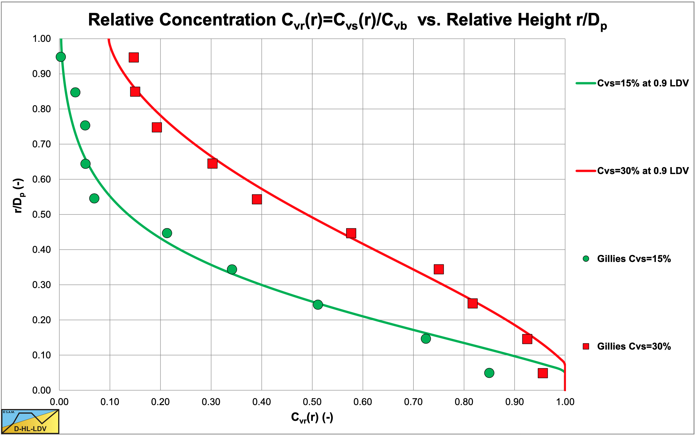
Figure 6.22-29 and Figure 6.22-30 show the concentration distributions for 2 average volumetric concentrations and 2 line speeds for a pipe diameter of Dp=0.0532 m and a particle diameter of d=2.4 m. The LDV (the line speed where there is no bed anymore) is about 2.0 m/s for a 17.5% volumetric concentration and slightly lower for the lower and higher concentrations. The fit lines are based on the DHLLDV Framework, assuming a bed concentration of 55%. So at a line speed of 1.8 m/s a bottom concentration close to the bed concentration is expected, but at 3.1 m/s above the LDV a lower bottom concentration and a slightly steeper concentration profile is expected.
In this chapter the concentration profiles in a Dp=0.0532 m pipe are compared with the data of Gillies (1993). In chapter 7.10 the concentration profiles in a Dp=0.263 m pipe are compared with the data of Gillies (1993). In both cases the predictions according to the DHLLDV Framework match well, although not perfect.
It should be mentioned that the LDV values used are an average based on the DHLLDV Framework, while the LDV is concentration dependent. The DHLLDV Framework is a bit conservative giving high values for the LDV.
6.22.12 Nomenclature SRC Model
|
Ar |
Archimedes number |
- |
|
Ap |
Cross section pipe |
m2 |
|
A1 |
Cross section above bed |
m2 |
|
A2 |
Cross section bed |
m2 |
|
Cvb |
Volumetric spatial bed concentration |
- |
|
Cvb,max |
Maximum volumetric spatial bed concentration |
- |
|
Cvs |
Spatial volumetric concentration |
- |
|
Cvs,1 |
Spatial volumetric concentration in cross section 1 |
- |
|
Cvs,2 |
Spatial volumetric concentration in cross section 2 |
- |
|
Cvs,c |
Spatial volumetric concentration in contact load |
- |
|
CD |
Particle drag coefficient |
- |
|
d |
Particle diameter |
m |
|
d+ |
Dimensionless particle diameter |
- |
|
d50 |
Particle diameter with 50% passing |
m |
|
DH |
Hydraulic diameter |
m |
|
Dp |
Pipe diameter |
m |
|
Erhg |
Relative excess hydraulic gradient |
- |
|
Fr |
Froude number |
- |
|
FL |
Durand & Condolios LDV Froude number |
- |
|
Fr |
Froude number |
- |
|
g |
Gravitational constant 9.81 m/s2 |
m/s2 |
|
il |
Hydraulic gradient liquid |
m/m |
|
im |
Hydraulic gradient mixture |
m/m |
|
ΔL |
Length of pipe section |
m |
|
LDV |
Limit Deposit Velocity |
m/s |
|
LSDV |
Limit of Stationary Deposit Velocity |
m/s |
|
Op |
Circumference pipe |
m |
|
O1 |
Circumference pipe above bed |
m |
|
O2 |
Circumference pipe in bed |
m |
|
O12 |
Width of bed |
m |
|
Δp |
Pressure difference |
kPa |
|
Δpl |
Pressure difference liquid |
kPa |
|
Δpm |
Pressure difference mixture |
kPa |
|
Re |
Reynolds number |
- |
|
Rsd |
Relative submerged density |
- |
|
u* |
Friction velocity |
m/s |
|
vt |
Terminal settling velocity |
m/s |
|
vls |
Line speed |
m/s |
|
vls,ldv |
Limit Deposit Velocity |
m/s |
|
v1 |
Cross section averaged velocity above bed |
m/s |
|
v2 |
Cross section averaged velocity bed |
m/s |
|
yb |
Height of bed |
m |
|
α |
Darcy Weisbach friction factor, multiplication factor |
- |
|
β |
Bed angle |
rad |
|
ε |
Pipe wall roughness |
m |
|
δv |
Thickness viscous sub layer |
m |
|
ρl |
Density carrier liquid |
ton/m3 |
|
ρs |
Density solids |
ton/m3 |
|
ρm1 |
Density in the upper layer |
ton/m3 |
|
ρm2 |
Density in the lower layer |
ton/m3 |
|
λlc |
Linear concentration |
- |
|
λl |
Darcy-Weisbach friction factor liquid-pipe wall |
- |
|
λ1 |
Darcy-Weisbach friction factor with pipe wall |
- |
|
λ2 |
Darcy-Weisbach friction factor with pipe wall, liquid in bed |
- |
|
λ12 |
Darcy-Weisbach friction factor on the bed |
- |
|
λs |
Solids effect to Darcy-Weisbach friction factor |
- |
| \(\ v_{\mathrm{l}}\) |
Kinematic viscosity |
m2/s |
| \(\ \tau_{\mathrm{l}}\) |
Shear stress liquid-pipe wall |
kPa |
| \(\ \tau_{1,\mathrm{l}}\) |
Shear stress liquid-pipe wall above bed |
kPa |
| \(\ \tau_{12,\mathrm{l}}\) |
Shear stress bed-liquid |
kPa |
| \(\ \tau_{2,\mathrm{l}}\) |
Shear stress liquid-pipe in bed |
kPa |
| \(\ \tau_{2,\mathrm{sf}}\) |
Shear stress from sliding friction |
kPa |
|
μsf |
Sliding friction coefficient |
- |
|
μsf0 |
Sliding friction coefficient, basic |
- |