
7.13: Influence of the Particle Size Distribution
- Page ID
- 32143

7.13.1 Introduction
The im curve for graded sands and gravels can be determined by:
- Determine the fraction fines X. The limiting particle diameter for the fines can be determined with equation (7.13-2).
- Determine the PSD and split the PSD in n fractions. Correct the PSD so the fines are not part of the PSD anymore. Adjust the volumetric concentration by deducting the fines fraction X.
- Adjust the pseudo liquid dynamic viscosity μx, density ρx and relative submerged density Rsd,x for the presence of fines and determine the resulting hydraulic gradient curve for the pseudo liquid, il,x.
- Determine curves related to the pseudo liquid.
- Determine the im,x,i curve for each ith fraction individually for both the spatial volumetric concentration and the delivered volumetric concentration, using the adjusted pseudo liquid properties.
- Sum the im,x,i curves for the n fractions multiplied by the fraction fi to determine the total hydraulic gradient im,x, for both the spatial volumetric concentration and the delivered volumetric concentration, in the pseudo liquid.
- Determine the resulting Erhg,x curve, for both the spatial volumetric concentration and the delivered volumetric concentration.
- Determine curves related to the carrier liquid.
- Determine the im,i curves for the n fractions by multiplying the im,x,i curves by the ratio of the pseudo liquid density to the carrier liquid density ρx/ρl.
- Sum the im,i curves for the n fractions multiplied by the fraction fi to determine the total hydraulic gradient im, for both the spatial volumetric concentration and the delivered volumetric concentration, in the carrier liquid.
- Determine the resulting Erhg curve, for both the spatial volumetric concentration and the delivered volumetric concentration.
- Determine the bed fraction curves for each fraction multiplied by the fraction fi.
- Sum the bed fraction curves for the n fractions multiplied by the fraction fi to obtain the total bed fraction curve.
- Determine the slip ratio curves for each fraction multiplied by the fraction fi.
- Sum the slip ratio curves for the n fractions multiplied by the fraction fi to obtain the total slip ratio curve.
Step 2 needs some clarification. Suppose we have a sand with 3 fractions, each 1/3 by weight. The first fraction consists of fines, the second fraction of particles with a d=0.5 mm and the third fraction of particles with d=1 mm. The spatial volumetric concentration of the sand in the carrier liquid is 30%.
Now the fines form a pseudo homogeneous liquid together with the carrier liquid. So in terms of solids effect they do not take part in the solids effect and have to be removed from the PSD. What is left is a PSD with 50% particles with a d=0.5 mm and 50% particles with d=1 mm. The spatial volumetric concentration of this sand is now 20%. So the hydraulic gradients have to be determined for this remaining sand and not for the original sand.
If a sand does not contain fines, the liquid properties and the PSD do not have to be adjusted.
7.13.2 The Adjusted Pseudo Liquid Properties
First the limiting particle diameter is determined, based on a Stokes number of 0.03. The value of 0.03 is found based on many experiments from literature. Since the Stokes number depends on the line speed, here the Limit Deposit Velocity is used as an estimate of the operational line speed.
The LDV is approximated by:
\[\ \mathrm{v}_{\mathrm{l s}, \mathrm{ld v}}=\mathrm{7 .5 \cdot} \mathrm{D}_{\mathrm{p}}^{\mathrm{0 . 4}}\]
Giving for the limiting particle diameter:
| \[\ \mathrm{d}_{\mathrm{lim}}=\sqrt{\frac{\mathrm{S t k} \cdot \mathrm{9} \cdot \rho_{\mathrm{l}} \cdot v_{\mathrm{l}} \cdot \mathrm{D}_{\mathrm{p}}}{\rho_{\mathrm{s}} \cdot \mathrm{v}_{\mathrm{l} \mathrm{s}, \mathrm{l} \mathrm{d} \mathrm{v}}}} \approx \sqrt{\frac{\mathrm{S t k} \cdot \mathrm{9} \cdot \rho_{\mathrm{l}} \cdot v_{\mathrm{l}} \cdot \mathrm{D}_{\mathrm{p}}}{\rho_{\mathrm{s}} \cdot \mathrm{7 . 5} \cdot \mathrm{D}_{\mathrm{p}}^{0.4}}}\] |
The fraction of the sand in suspension, resulting in a homogeneous pseudo fluid is named X. This gives for the density of the homogeneous pseudo fluid:
| \[\ \rho_{\mathrm{x}}=\rho_{\mathrm{l}}+\rho_{\mathrm{l}} \cdot \frac{\mathrm{X} \cdot \mathrm{C}_{\mathrm{v} \mathrm{s}} \cdot \mathrm{R}_{\mathrm{s d}}}{\left(\mathrm{1}-\mathrm{C}_{\mathrm{v s}}+\mathrm{C}_{\mathrm{v s}} \cdot \mathrm{X}\right)} \quad\text{ if }\quad\mathrm{X}=\mathrm{1} \quad \Rightarrow \quad \rho_{\mathrm{x}}=\rho_{\mathrm{m}}=\rho_{\mathrm{l}}+\rho_{\mathrm{l}} \cdot \mathrm{C}_{\mathrm{v} \mathrm{s}} \cdot \mathrm{R}_{\mathrm{s} \mathrm{d}}\] |
So the concentration of the homogeneous pseudo fluid is not Cvs,x=X·Cvs, but:
| \[\ \mathrm{C}_{\mathrm{v s}, \mathrm{x}}=\frac{\mathrm{X} \cdot \mathrm{C}_{\mathrm{v s}}}{\left(1-\mathrm{C}_{\mathrm{v s}}+\mathrm{C}_{\mathrm{v s}} \cdot \mathrm{X}\right)}\] |
This is because part of the total volume is occupied by the particles that are not in suspension. The remaining spatial concentration of solids to be used to determine the individual hydraulic gradients curves of the fractions is now:
| \[\ \mathrm{C}_{\mathrm{v s}, \mathrm{r}}=(\mathrm{1}-\mathrm{X}) \cdot \mathrm{C}_{\mathrm{v s}}\] |
The dynamic viscosity can now be determined according to Thomas (1965):
| \[\ \mu_{\mathrm{x}}=\mu_{\mathrm{l}} \cdot\left(1+\mathrm{2 .5} \cdot \mathrm{C}_{\mathrm{v s}, \mathrm{x}}+\mathrm{1 0 . 0 5} \cdot \mathrm{C}_{\mathrm{v s}, \mathrm{x}}^{\mathrm{2}}+\mathrm{0 .0 0 2 7 3 \cdot} \mathrm{e}^{\mathrm{1 6 . 6} \cdot \mathrm{C}_{\mathrm{v s}, \mathrm{x}}}\right)\] |
The kinematic viscosity of the homogeneous pseudo fluid is now:
| \[\ v_{\mathrm{x}}=\frac{\mu_{\mathrm{x}}}{\rho_{\mathrm{x}}}\] |
One should realize however that the relative submerged density has also changed to:
| \[\ \mathrm{R}_{\mathrm{s d}, \mathrm{x}}=\frac{\rho_{\mathrm{s}}-\rho_{\mathrm{x}}}{\rho_{\mathrm{x}}}\] |
With the new homogeneous pseudo liquid density, kinematic viscosity, relative submerged density and volumetric concentration the hydraulic gradient can be determined for each fraction of the adjusted PSD.
7.13.3 A Method To Generate a PSD
The original fractions of the PSD can be determined manually by sieve analysis, or generated based on for example the d50/d15 and d85/d50 ratios. A mathematical function describing the shape of a PSD up to the d50 is:
\[\ \mathrm{f_{y}={\frac{1}{1+e^{A_{x}\cdot\left(\frac{\log 10\left(d_{y}\right)}{\log 10\left(d_{50}\right)}-1\right)}}} \quad\text{ with: }\quad A_{x}=\frac{1}{\left(\frac{\log 10\left(d_{x}\right)}{\log 10\left(d_{50}\right)}-1\right)} \cdot \ln \left(\frac{1-f_{x}}{f_{x}}\right)}\]
Now suppose:
\[\ \alpha_{15}=\frac{\mathrm{d}_{50}}{\mathrm{d}_{15}} \quad\text{ and }\quad \alpha_{85}=\frac{\mathrm{d}_{85}}{\mathrm{d}_{50}}\]
This gives:
\[\ \begin{array}{left} \mathrm{A_{15}}&=\mathrm{\frac{1}{\left(\frac{log10(d_{15})}{log10(d_{50})}-1 \right)}\cdot ln \left(\frac{1-0.15}{0.15} \right)=\frac{1}{\left(\frac{log10\left(\frac{d_{50}}{\alpha_{15}} \right)}{log10(d_{50})}-1 \right)}\cdot ln\left(\frac{0.85}{0.15} \right)}\\
&=\mathrm{-\frac{log10(d_{50})}{log10(\alpha_{15})}\cdot ln \left(\frac{0.85}{0.15} \right)=-1.7346\cdot\frac{ln(d_{50})}{ln(\alpha_{15})}}\end{array}\]
\[\ \begin{array}{left}\mathrm{A_{85}}&=\mathrm{-\frac{1}{\left(\frac{log10(d_{85})}{log10(d_{50})}-1 \right)}\cdot ln\left(\frac{1-0.85}{0.85} \right)=\frac{1}{\left(\frac{log10(\alpha_{85}\cdot d_{50})}{log10 (d_{50})}-1 \right)}\cdot ln\left(\frac{0.85}{0.15} \right)}\\
&=\mathrm{-\frac{log10(d_{50})}{log10(\alpha_{85})}\cdot ln\left(\frac{0.85}{0.15} \right)=-1.7346 \cdot \frac{ln(d_{50})}{ln(\alpha_{85})}}
\end{array} \]
Now suppose for the ratios d50/d15 and d85/d50:
\[\ \alpha_{15}=\frac{\mathrm{d}_{50}}{\mathrm{d}_{15}}=\mathrm{e}^{1}=2.7183 \quad\text{ and }\quad \alpha_{85}=\frac{\mathrm{d}_{85}}{\mathrm{d}_{50}}=\mathrm{e}^{1}=2.71 \mathrm{8 3}\]
This gives for A15 and A85 positive values as long as the d50<1 m:
\[\ \begin{array}{left}\mathrm{A_{15}=-1.7346 \cdot ln(d_{50})}\\
\mathrm{A_{85}=-1.7346 \cdot ln(d_{50})}
\end{array}\]
So the fraction passing in the PSD is in this particular symmetrical case:
\[\ \mathrm{f}_{\mathrm{y}}=\frac{\mathrm{1}}{1+\mathrm{e}^{\mathrm{A}_{15} \cdot\left(\frac{\log 10\left(\mathrm{d}_{\mathrm{y}}\right)}{\log 10\left(\mathrm{d}_{50}\right)}-1\right)}}=\frac{\mathrm{1}}{1+\mathrm{e}^{\mathrm{A}_{85} \cdot\left(\frac{\log 10\left(\mathrm{d}_{\mathrm{y}}\right)}{\log 10\left(\mathrm{d}_{50}\right)}-1\right)}}=\frac{1}{1+\mathrm{e}^{-1.7346 \cdot \left(\mathrm{ln(d_y)-ln(d_{50})} \right)}}\]
Of course there are other ways to generate PSD’s, but this way works well and gives the possibility to create an asymmetrical PSD if α15 and α85 are chosen differently.
7.13.4 Determination of the Hydraulic Gradient
After adjusting for the new homogeneous pseudo liquid density ρx, kinematic viscosity \(\ v_{\mathrm{x}} \) and relative submerged density Rsd,x the hydraulic gradient can be determined for each fraction of the adjusted PSD using the volumetric concentration of the remaing solids. It is important to determine the hydraulic gradient curve for the full velocity range for both spatial and delivered concentrations and not the relative excess hydraulic gradient curves. The reason is, that the hydraulic gradient curves include the liquid curve for the adjusted homogeneous pseudo fluid properties, while the relative excess hydraulic gradient curves don’t. Later the relative excess hydraulic gradient curves can be determined using the hydraulic gradient of the pure carrier liquid and the relative submerged density of the solids in the pure carrier liquid.
The resulting hydraulic gradient im based on the pseudo liquid and relative excess hydraulic gradient Erhg are:
| \[\ \begin{array}{left}\mathrm{i}_{\mathrm{m}, \mathrm{x}}=\sum_{\mathrm{i}=\mathrm{1}}^{\mathrm{n}} \mathrm{f}_{\mathrm{i}} \cdot \mathrm{i}_{\mathrm{m}, \mathrm{x}, \mathrm{i}} \cdot \mathrm{w}_{\mathrm{i}} \quad \text { with: }\quad \sum_{\mathrm{i}=\mathrm{1}}^{\mathrm{n}} \mathrm{f}_{\mathrm{i}}=\mathrm{1} \quad \text { and } \quad \frac{\mathrm{1}}{\mathrm{n}} \cdot \sum_{\mathrm{i}=\mathrm{1}}^{\mathrm{n}} \mathrm{w}_{\mathrm{i}}=\mathrm{1} \\ \mathrm{E}_{\mathrm{r h g}, \mathrm{x}}=\frac{\mathrm{i}_{\mathrm{m}, \mathrm{x}}-\mathrm{i}_{\mathrm{l}, \mathrm{x}}}{\mathrm{R}_{\mathrm{s d}, \mathrm{x}} \cdot \mathrm{C}_{\mathrm{v s}}} \quad \mathrm{o r} \quad \mathrm{E}_{\mathrm{r h g}, \mathrm{x}}=\frac{\mathrm{i}_{\mathrm{m}, \mathrm{x}}-\mathrm{i}_{\mathrm{l}, \mathrm{x}}}{\mathrm{R}_{\mathrm{s d}, \mathrm{x}} \cdot \mathrm{C}_{\mathrm{v t}}}\end{array}\] |
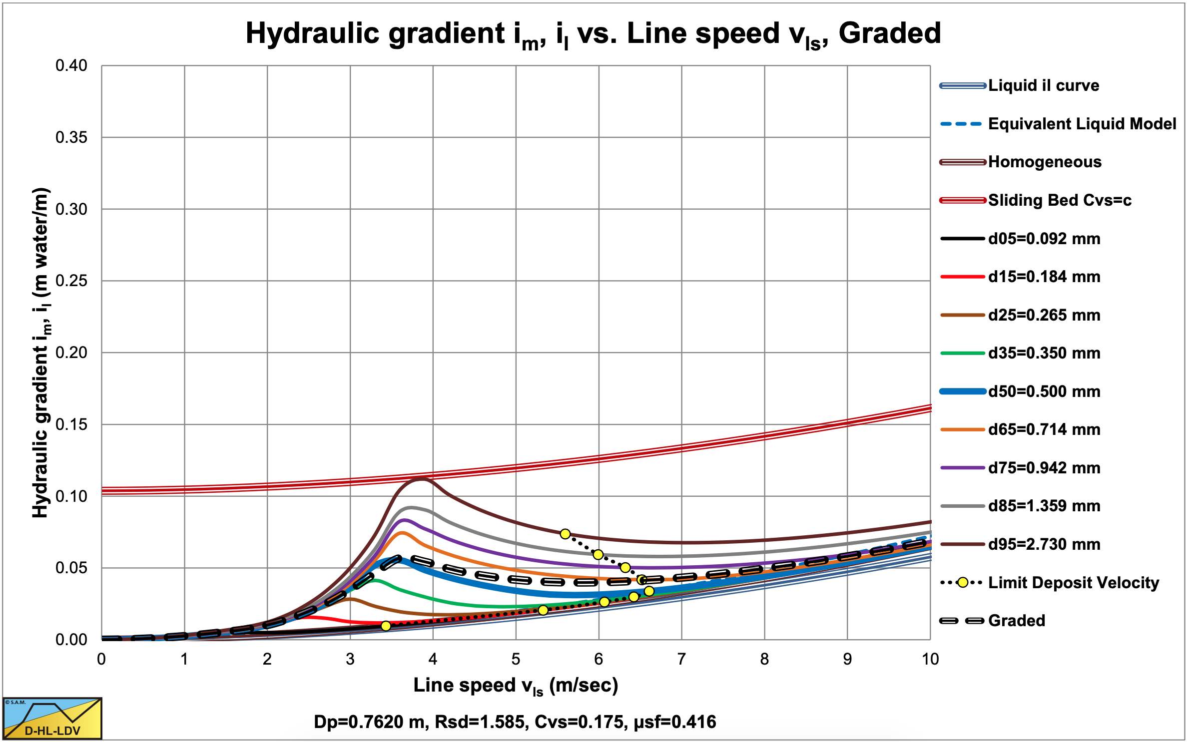
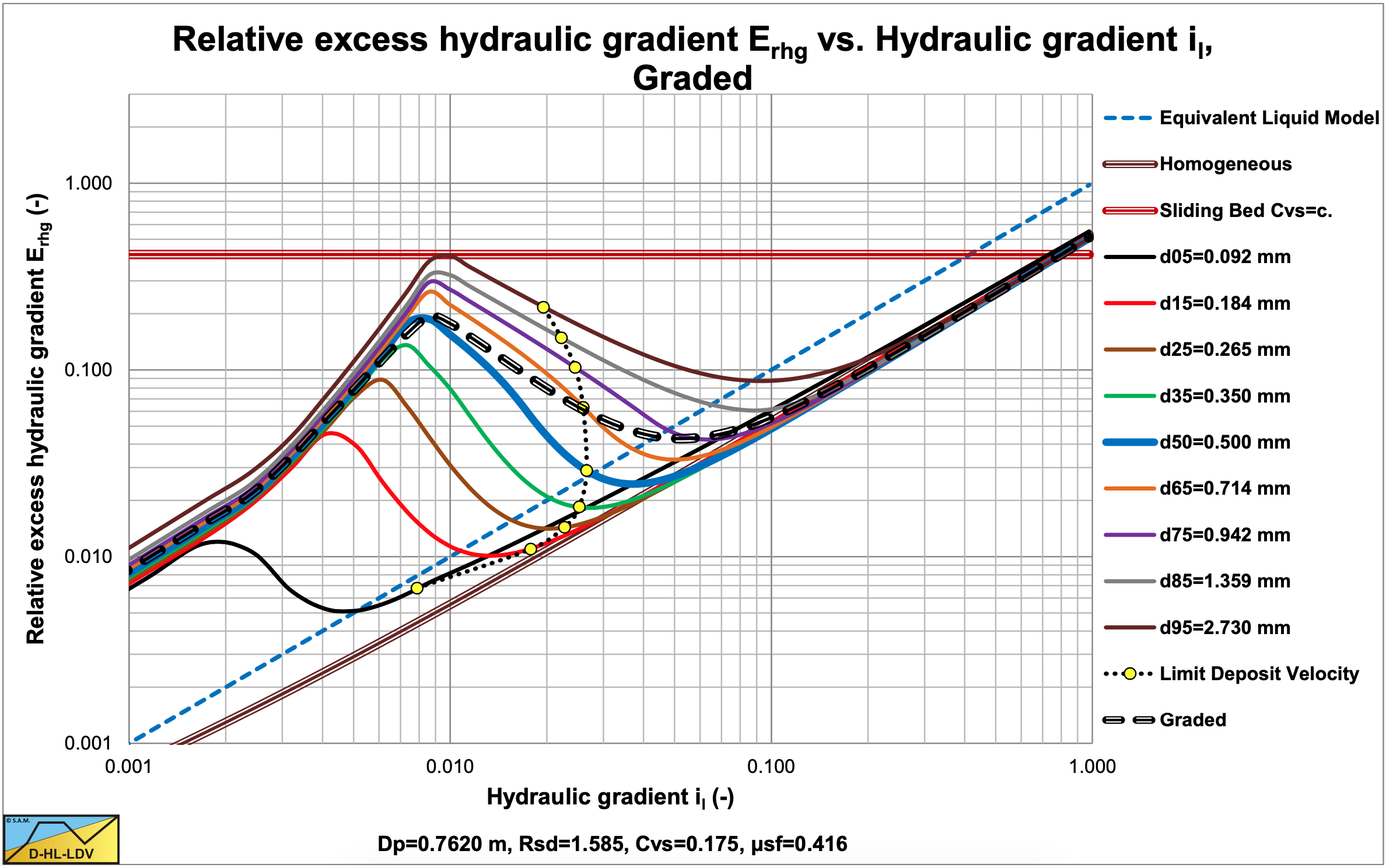
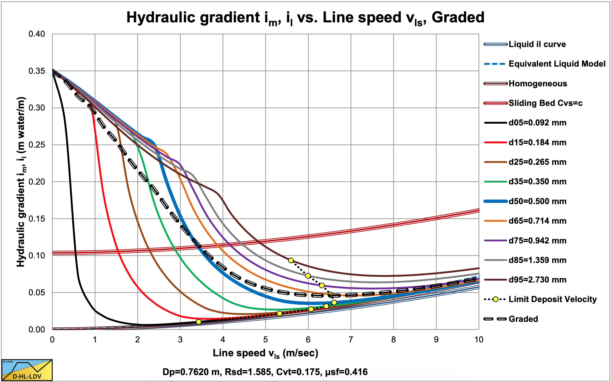
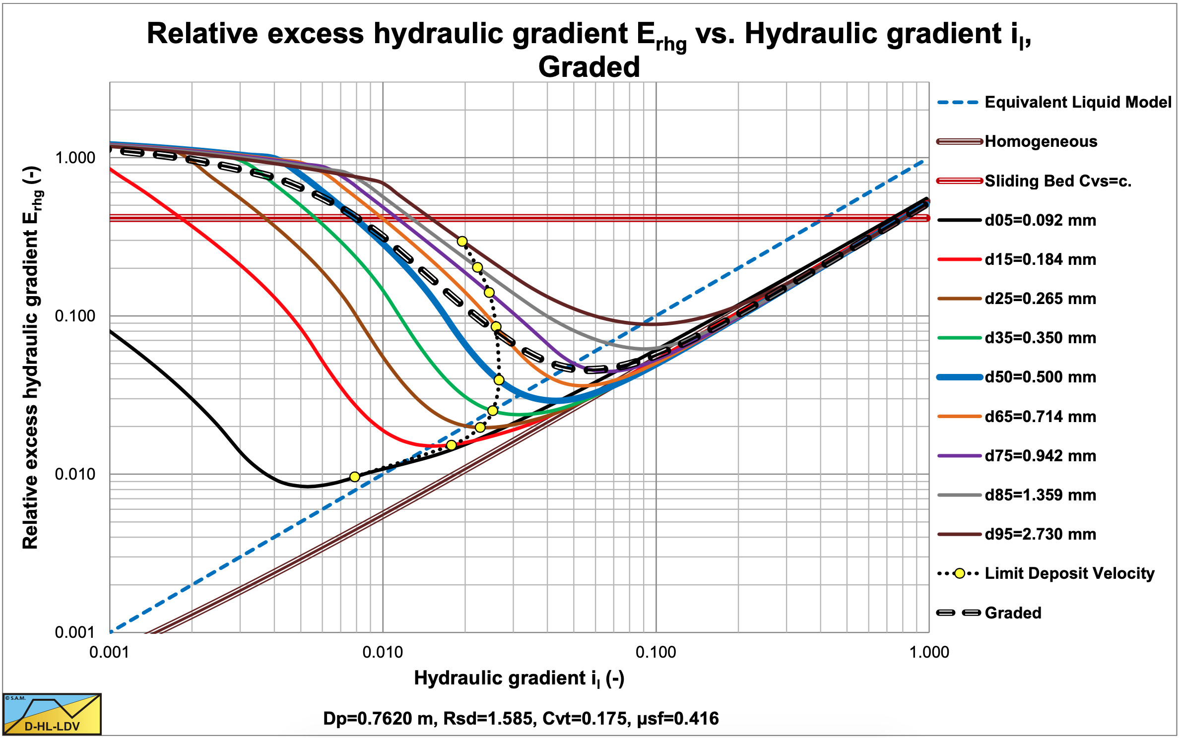
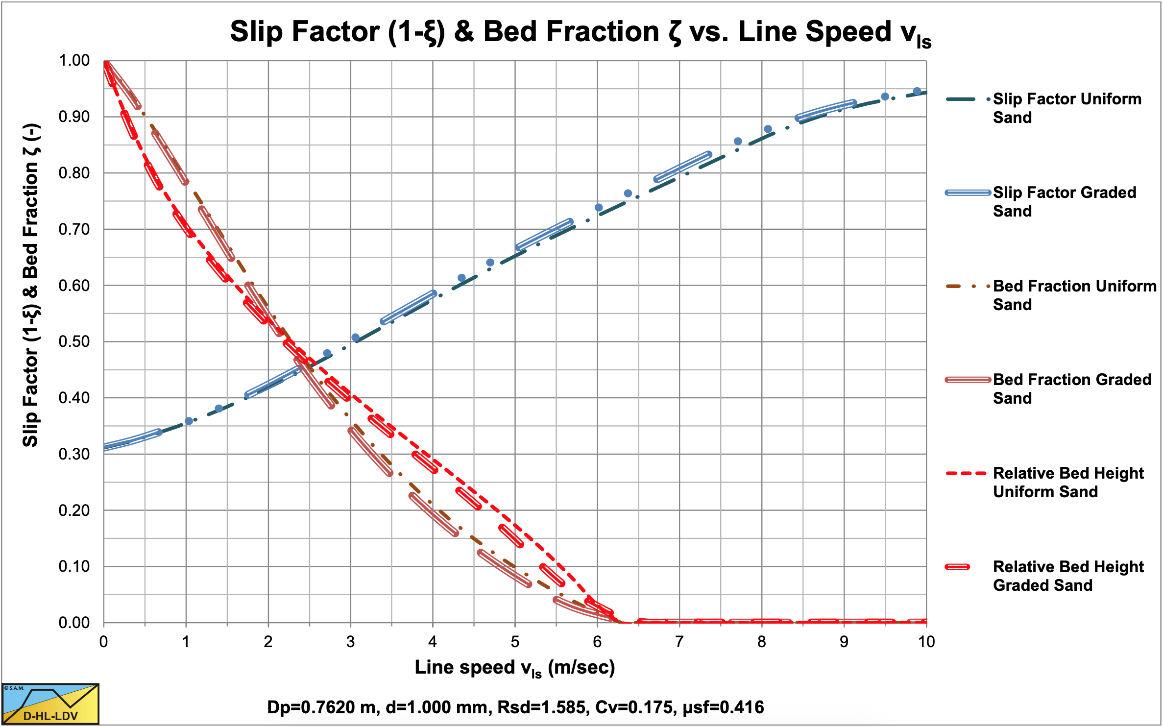
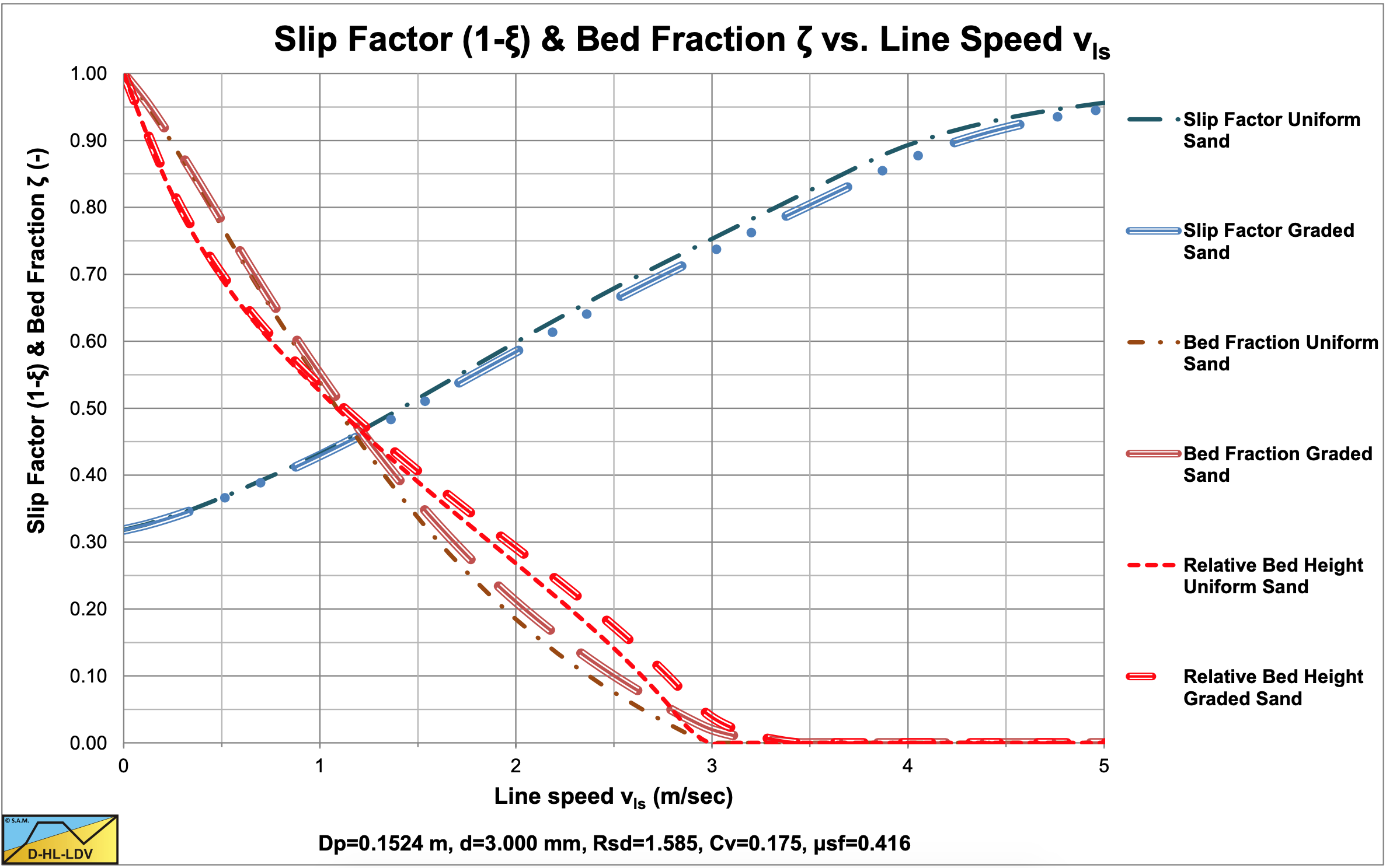
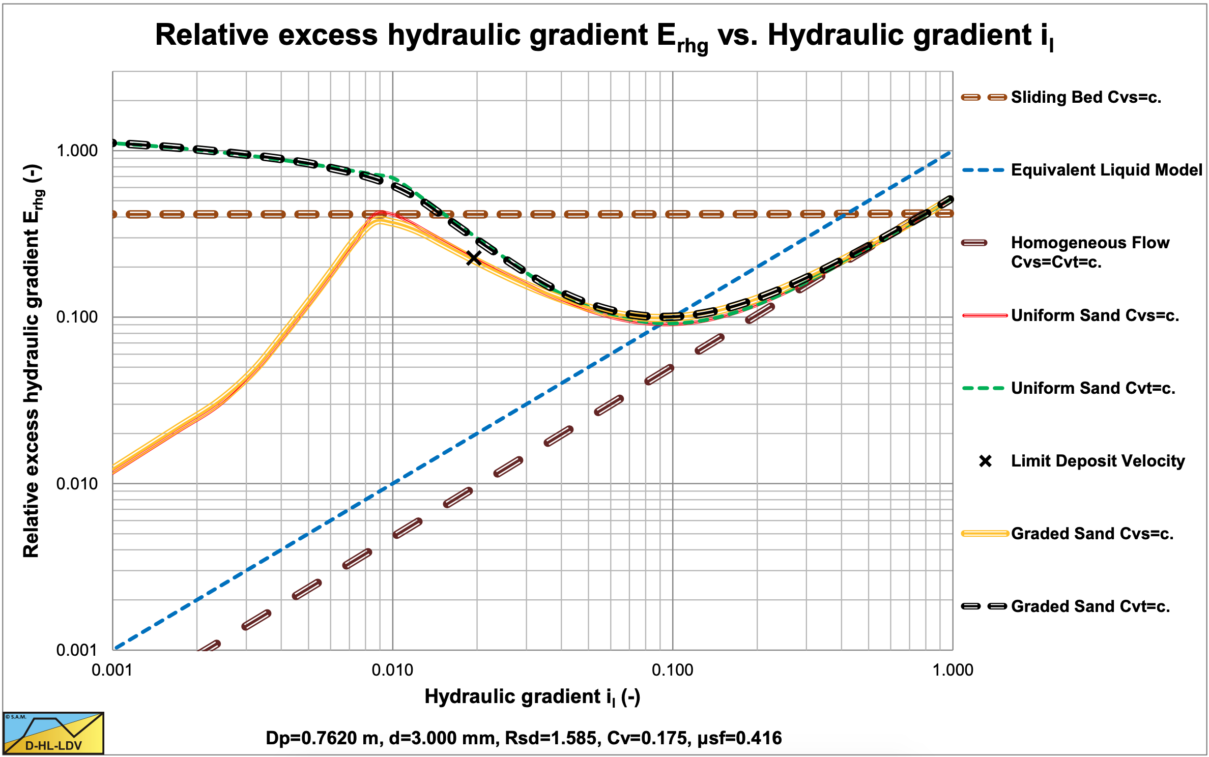
These are shown in Figure 7.13-1, Figure 7.13-2, Figure 7.13-3 and Figure 7.13-4 for 9 fractions. The thick blue lines show the curves for the d50 (uniform sand), while the black dashed lines show the resulting curves by adding up the curves of each fraction, giving the curve for graded sand. From Figure 7.13-2 and Figure 7.13-4 it is clear that the curve for graded sand is less steep than the curve for uniform sand. In Figure 7.13-4 there is an intersection point between the two curves which in fact is the v50 point of the Wilson et al. (1992) theory. The graded curve will sort of pivot around this point and be less steep the more graded the sand. Uniform sand will, of course follow the blue d50 curve, which is the steepest. It must be noted that the method described here follows the same trend as the Wilson et al. (1992) theory, but not exactly the same steepness is found. The shape of the graded curve also strongly depends on the particle and pipe diameter.
The resulting hydraulic gradient im,x based on the original carrier liquid and relative excess hydraulic gradient Erhg,x are:
| \[\ \begin{array}{left}\mathrm{i}_{\mathrm{m}}=\frac{\rho_{\mathrm{x}}}{\rho_{\mathrm{l}}} \cdot \mathrm{i}_{\mathrm{m}, \mathrm{x}}=\frac{\rho_{\mathrm{x}}}{\rho_{\mathrm{l}}} \cdot \sum_{\mathrm{i}=1}^{\mathrm{n}} \mathrm{f}_{\mathrm{i}} \cdot \mathrm{i}_{\mathrm{m}, \mathrm{x}, \mathrm{i}} \cdot \mathrm{w}_{\mathrm{i}} \quad\text{ with: }\quad \sum_{\mathrm{i}=1}^{\mathrm{n}} \mathrm{f}_{\mathrm{i}}=\mathrm{1} \quad\text{ and }\quad \frac{\mathrm{1}}{\mathrm{n}} \cdot \sum_{\mathrm{i}=\mathrm{1}}^{\mathrm{n}} \mathrm{w}_{\mathrm{i}}=\mathrm{1}\\ \mathrm{E}_{\mathrm{r h g}}=\frac{\mathrm{i}_{\mathrm{m}}-\mathrm{i}_{\mathrm{l}}}{\mathrm{R}_{\mathrm{s d}} \cdot \mathrm{C}_{\mathrm{v s}}} \quad\text{ or }\quad \mathrm{E}_{\mathrm{r h g}}=\frac{\mathrm{i}_{\mathrm{m}}-\mathrm{i}_{\mathrm{l}}}{\mathrm{R}_{\mathrm{s d}} \cdot \mathrm{C}_{\mathrm{v t}}}\end{array}\] |
The variable wi is a weighing factor, enabling to give certain particle diameters more weight in the total hydraulic gradient. Here the weighing factors are set to 1.
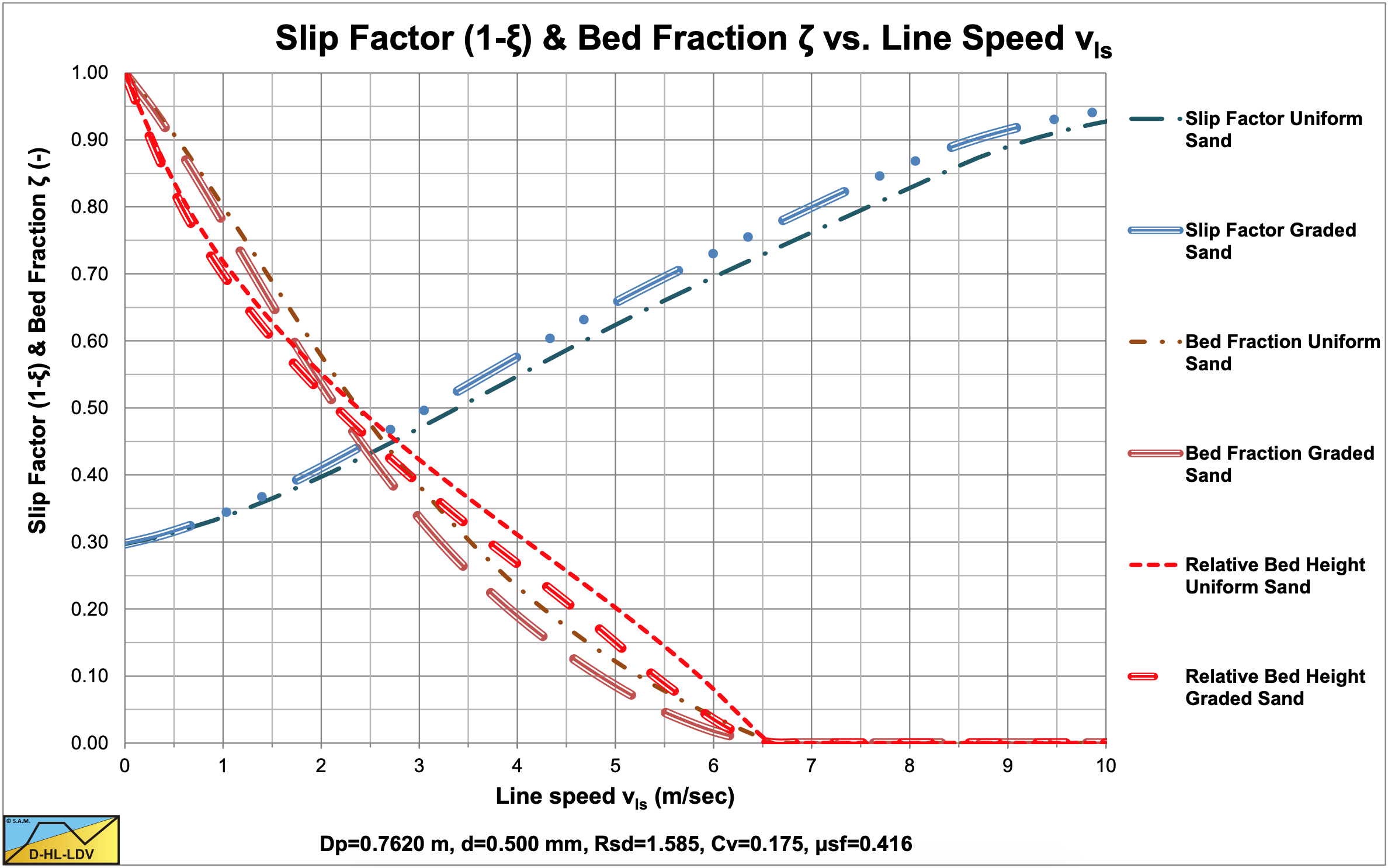
The resulting bed fraction is:
| \[\ \zeta=\tilde{\mathrm{A}}_{\mathrm{b}}=\sum_{\mathrm{i}=1}^{\mathrm{n}} \mathrm{f}_{\mathrm{i}} \cdot \tilde{\mathrm{A}}_{\mathrm{b}, \mathrm{i}}=\sum_{\mathrm{i}=1}^{\mathrm{n}} \mathrm{f}_{\mathrm{i}} \cdot \zeta_{\mathrm{i}} \quad\text{ with: }\sum_{\mathrm{i}=1}^{\mathrm{n}} \mathrm{f}_{\mathrm{i}}=1\] |
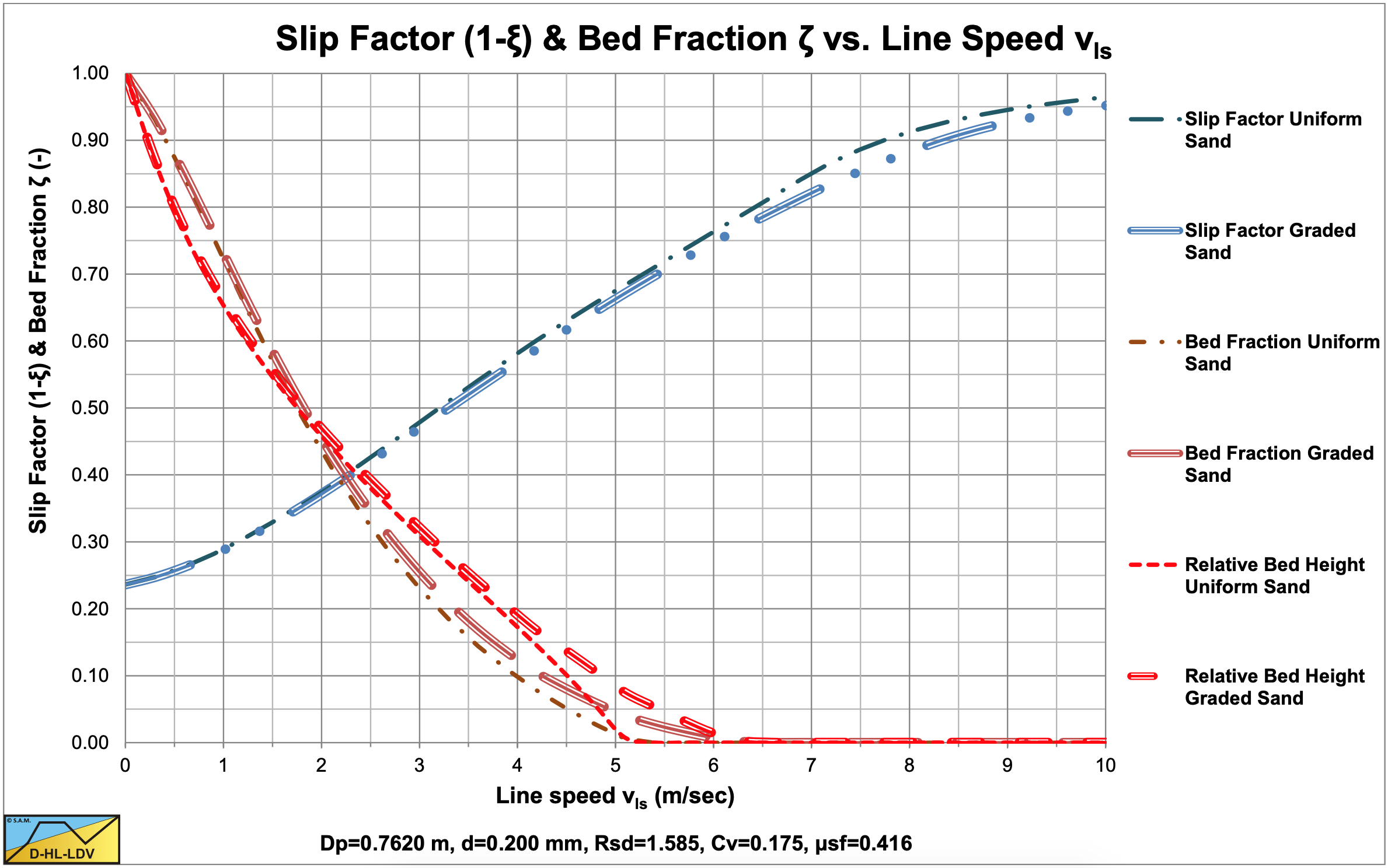
In the next sub-chapters examples are given for 4 particle diameters, d50, and 1 grading in a Dp=0.1524 m (6 inch) pipe and a Dp=0.762 m (30 inch) pipe. The choice of the particle diameters is such that the particle diameter of 0.2 mm will have a fines fraction influencing the liquid properties. First the 4 PSD’s are shown for d50=0.2 mm, d50=0.5 mm, d50=1.0 mm and d50=3.0 mm. The ratios d50/d15 and d85/d50 are set to 2.7183 as in the above equations. So the grading of each of the 4 sands is the same. For each sand the resulting relative excess hydraulic gradient curve, and the slip ratio/bed height curves are shown for both pipe diameters. The interpretation and conclusion are given below the graphs.
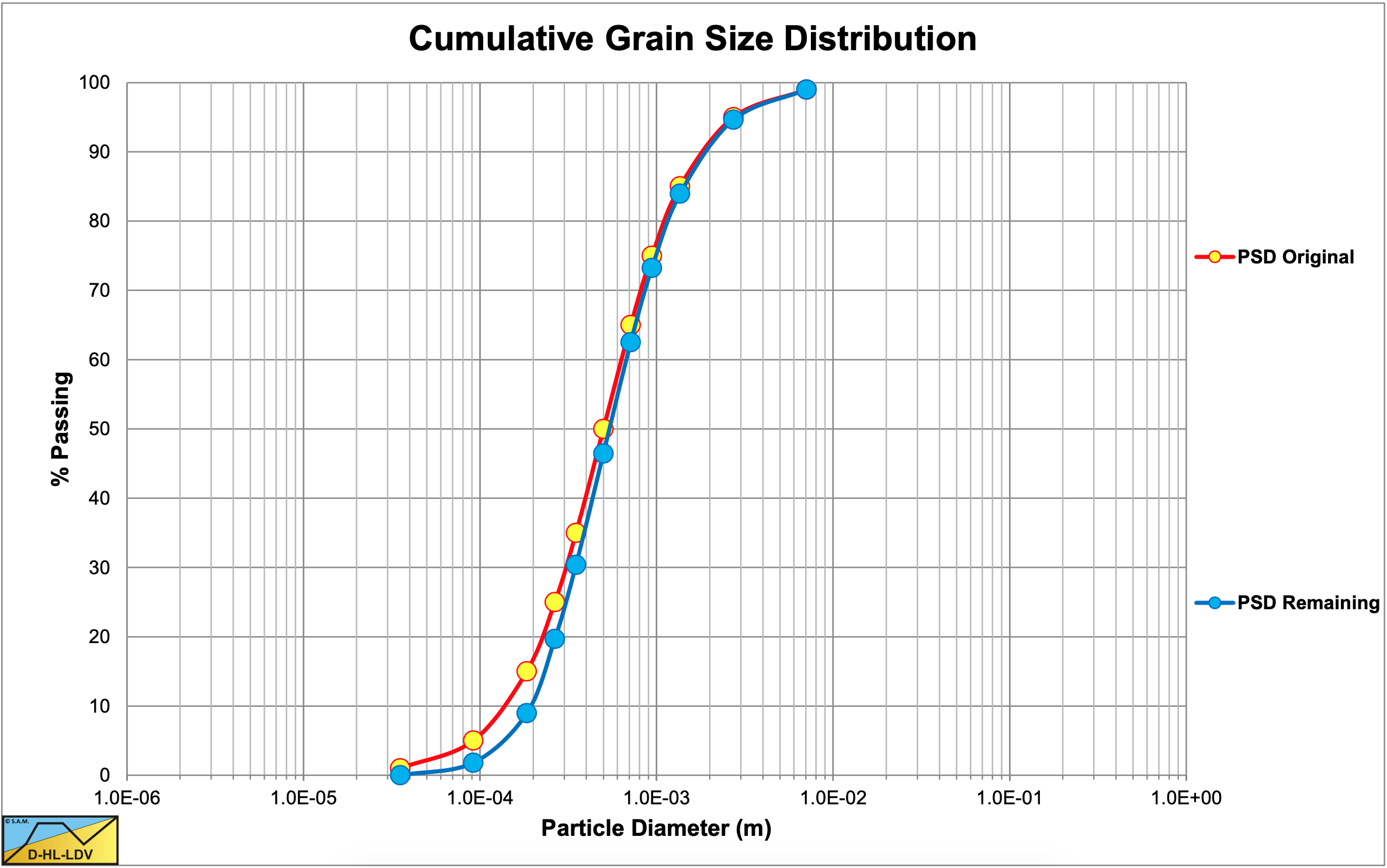
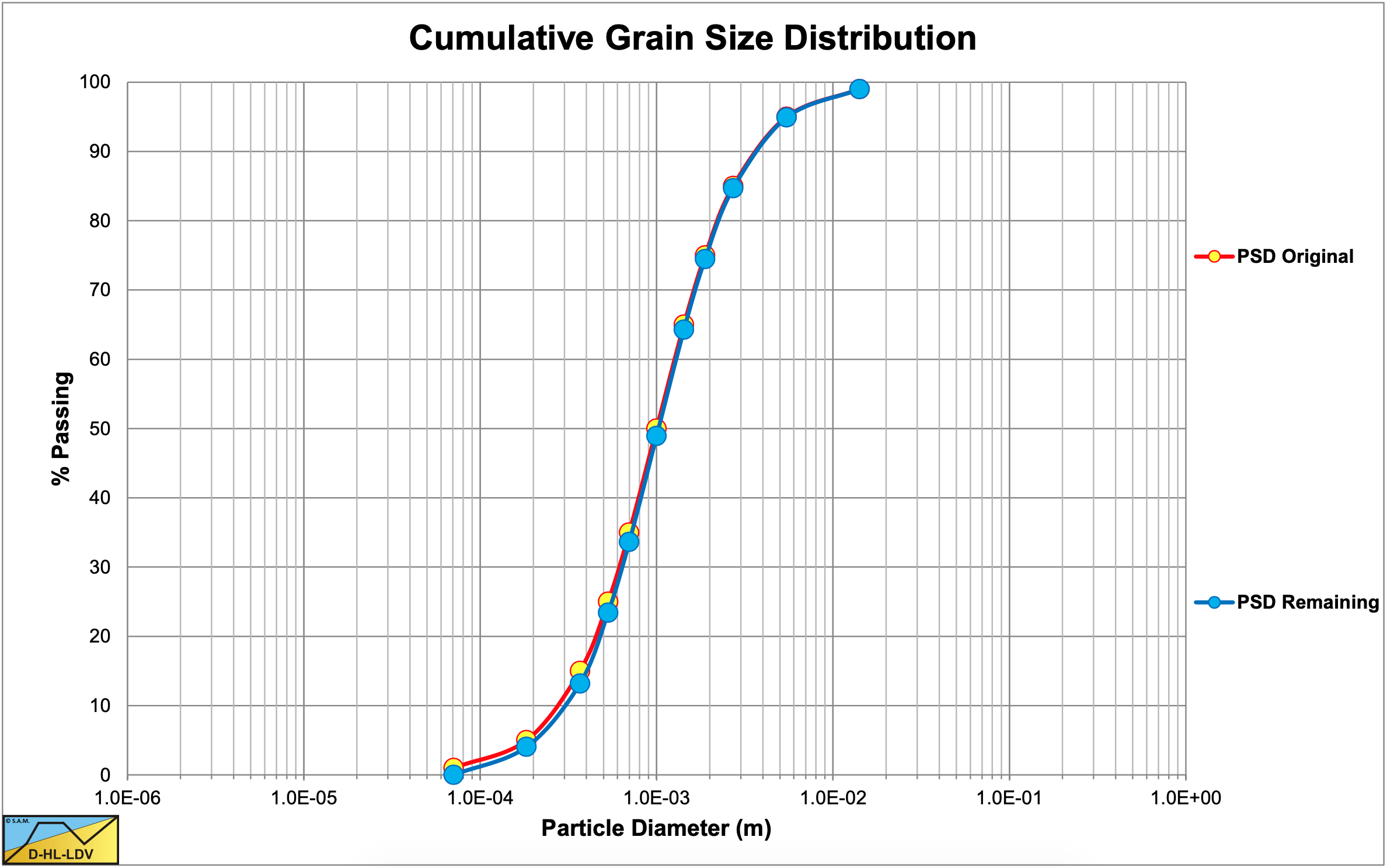
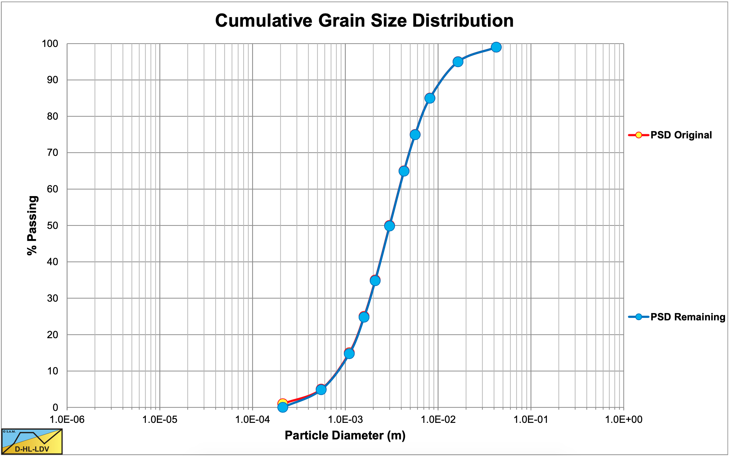
7.13.5 The Particle Size Distributions
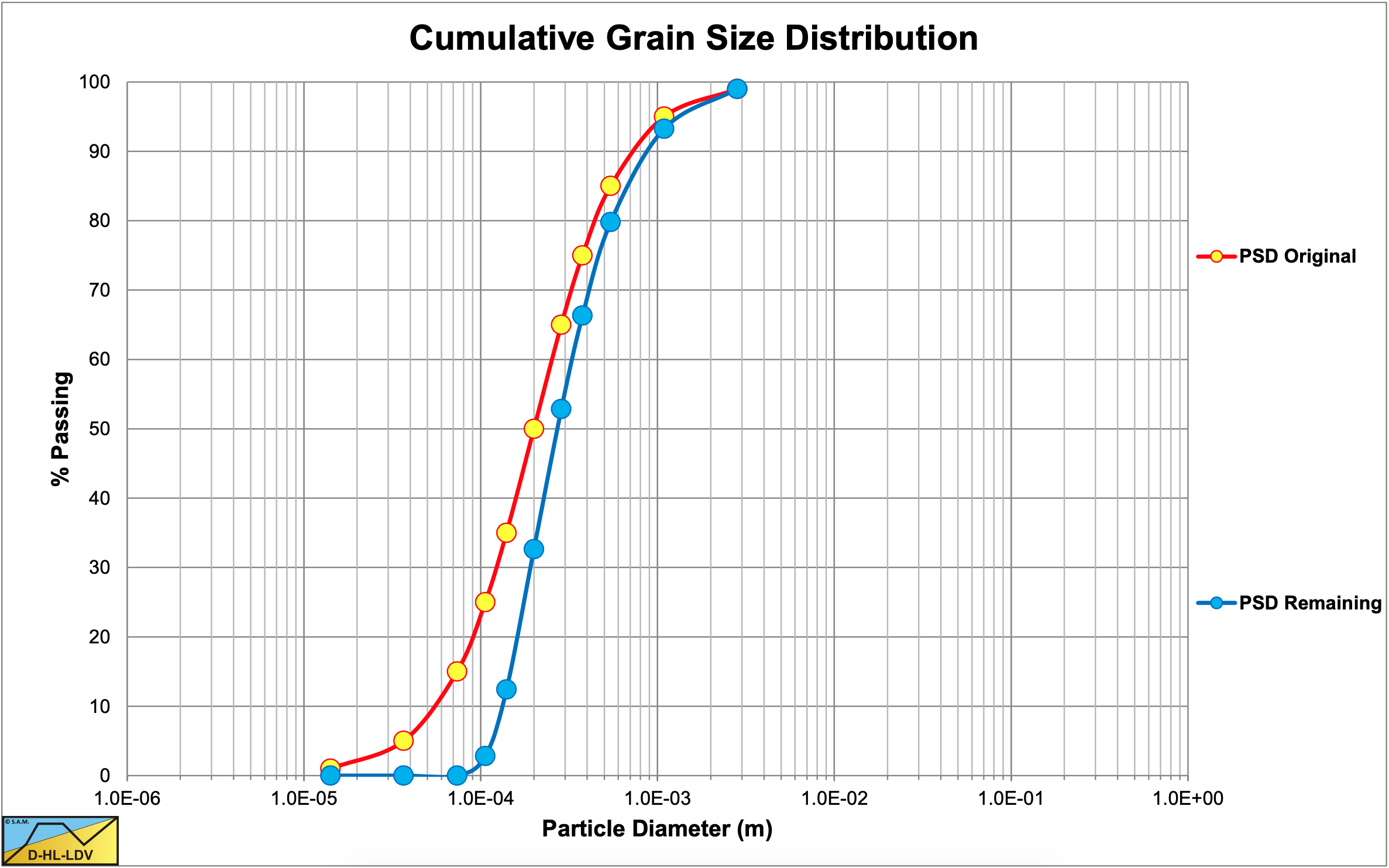
7.13.6 Particle Diameter d50=0.2 mm
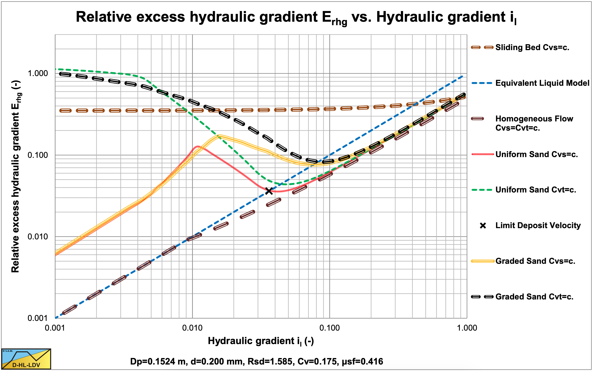

The values for A15 and A85 are 14.78. The graded relative excess hydraulic gradient curves are higher than the uniform curves in the operational range of hydraulic gradients (0.01-0.1). In the homogeneous region, the curves are higher than the theoretical homogeneous curve, because of the adjusted pseudo fluid properties. The fines diameter is d=0.067 mm and the percentage fines is 13.07% of the solids. The bed of the graded sand is lower than the bed of the uniform sand.
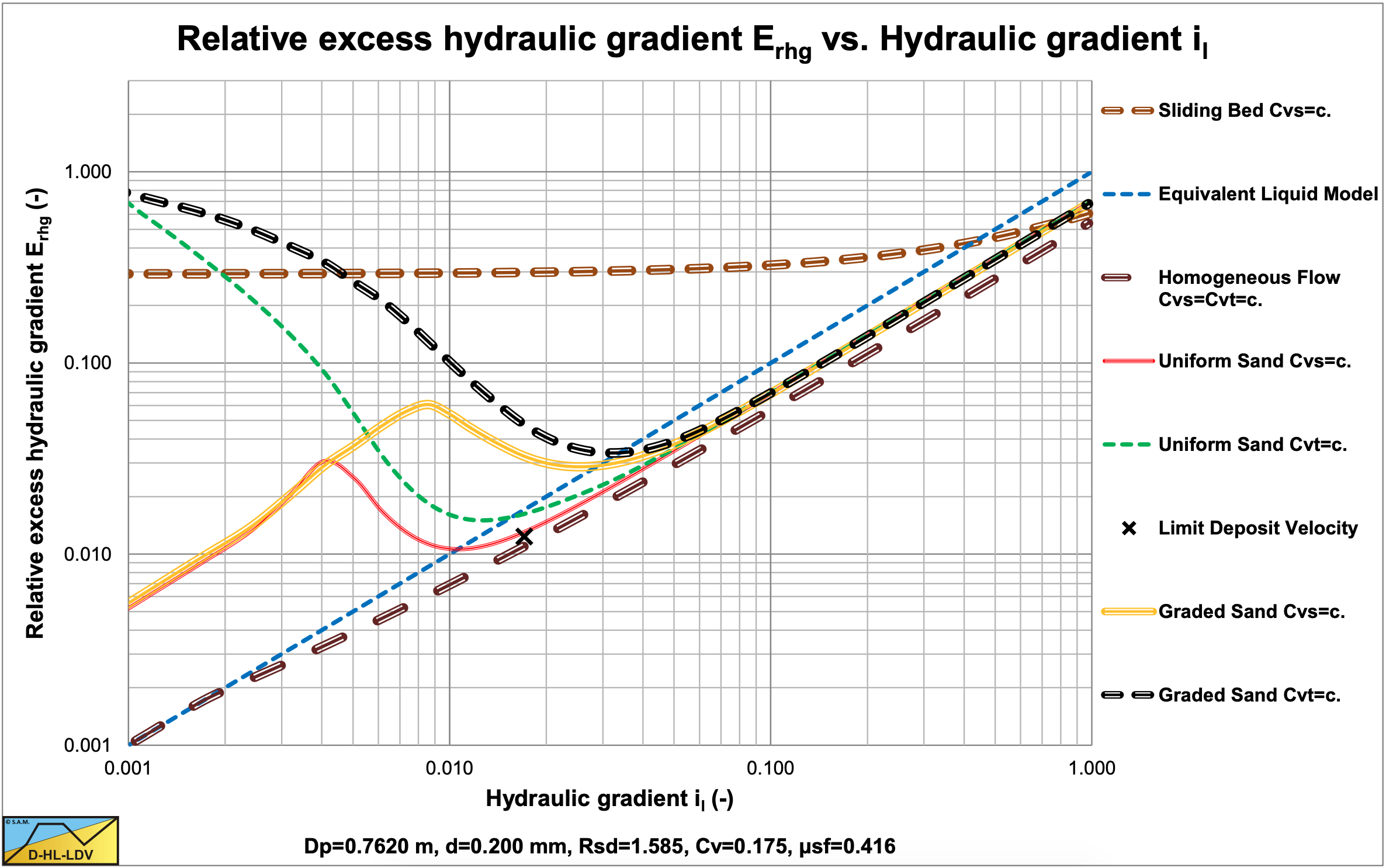
The values for A15 and A85 are 14.78. The graded relative excess hydraulic gradient curves are higher than the uniform curves in the operational range of hydraulic gradients (0.01-0.1). In the homogeneous region, the curves are higher than the theoretical homogeneous curve, because of the adjusted pseudo fluid properties. The fines diameter is d=0.109 mm and the percentage fines is 25.79% of the solids. The bed of the graded sand is lower than the bed of the uniform sand. A larger pipe gives a larger fines diameter and a larger fines fraction.
7.13.7 Particle Diameter d50=0.5 mm
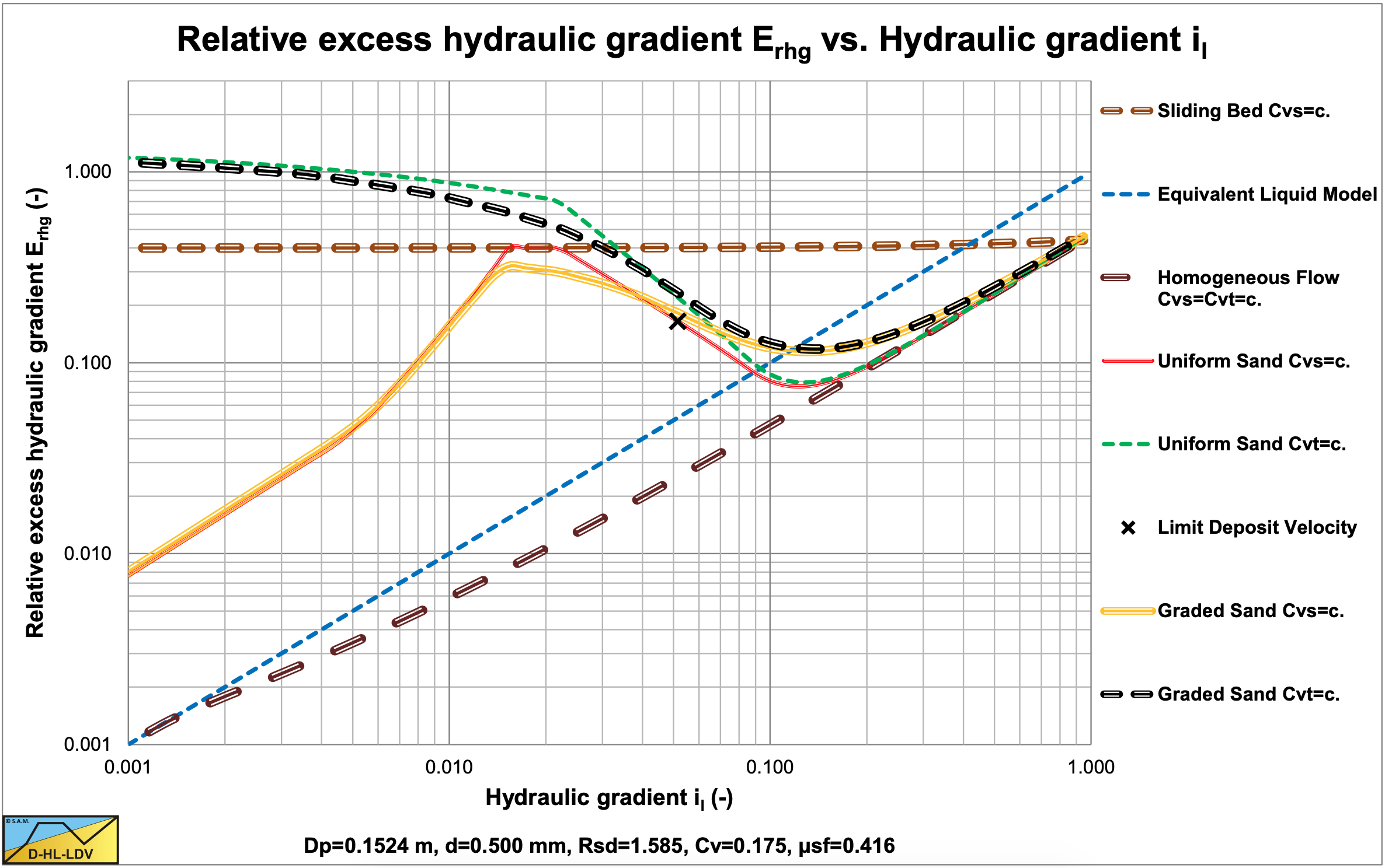

The values for A15 and A85 are 13.19. The graded relative excess hydraulic gradient curves are higher than the uniform curves in the operational range of hydraulic gradients (0.01-0.1). In the homogeneous region, the curves are slightly higher than the theoretical homogeneous curve, because of the adjusted pseudo fluid properties. The fines diameter is d=0.067 mm and the percentage fines is 2.98% of the solids. The bed of the graded sand is lower than the bed of the uniform sand.
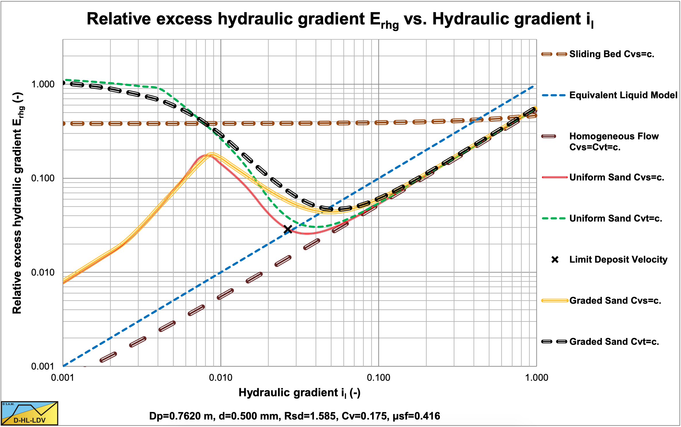
The values for A15 and A85 are 13.19. The graded relative excess hydraulic gradient curves are higher than the uniform curves in the operational range of hydraulic gradients (0.01-0.1). In the homogeneous region, the curves are slightly higher than the theoretical homogeneous curve, because of the adjusted pseudo fluid properties. The fines diameter is d=0.109 mm and the percentage fines is 6.62% of the solids. The bed of the graded sand is lower than the bed of the uniform sand. A larger pipe gives a larger fines diameter and a larger fines fraction.
7.13.8 Particle Diameter d50=1.0 mm
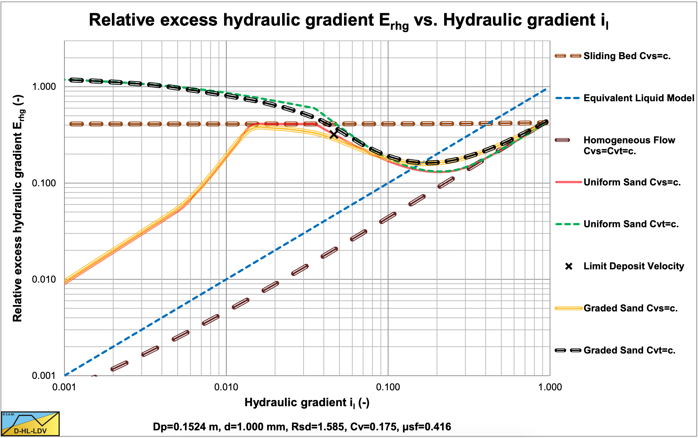

The values for A15 and A85 are 11.98. The graded relative excess hydraulic gradient curves are slightly higher than the uniform curves in the operational range of hydraulic gradients (0.01-0.1). In the homogeneous region, the curves are hardly higher than the theoretical homogeneous curve, because of the adjusted pseudo fluid properties. The fines diameter is d=0.067 mm and the percentage fines is 0.91% of the solids. The bed of the graded sand is hardly lower than the bed of the uniform sand.
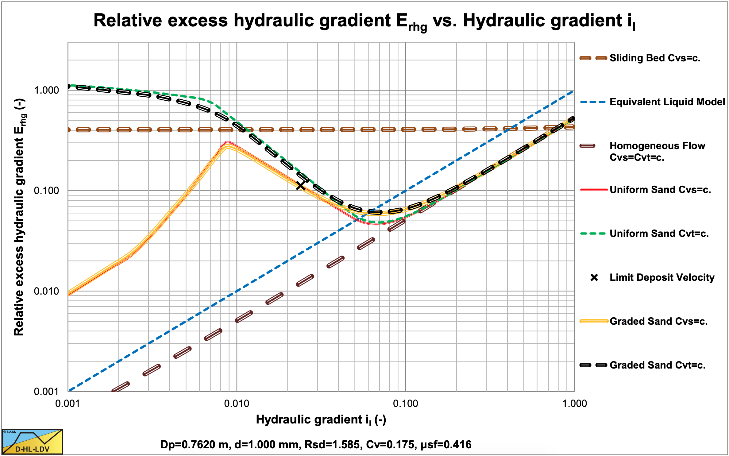
The values for A15 and A85 are 11.98. The graded relative excess hydraulic gradient curves are slightly higher than the uniform curves in the operational range of hydraulic gradients (0.01-0.1). In the homogeneous region, the curves are hardly higher than the theoretical homogeneous curve, because of the adjusted pseudo fluid properties. The fines diameter is d=0.109 mm and the percentage fines is 2.09% of the solids. The bed of the graded sand is hardly lower than the bed of the uniform sand. A larger pipe gives a larger fines diameter and a larger fines fraction.
7.13.9 Particle Diameter d50=3.0 mm
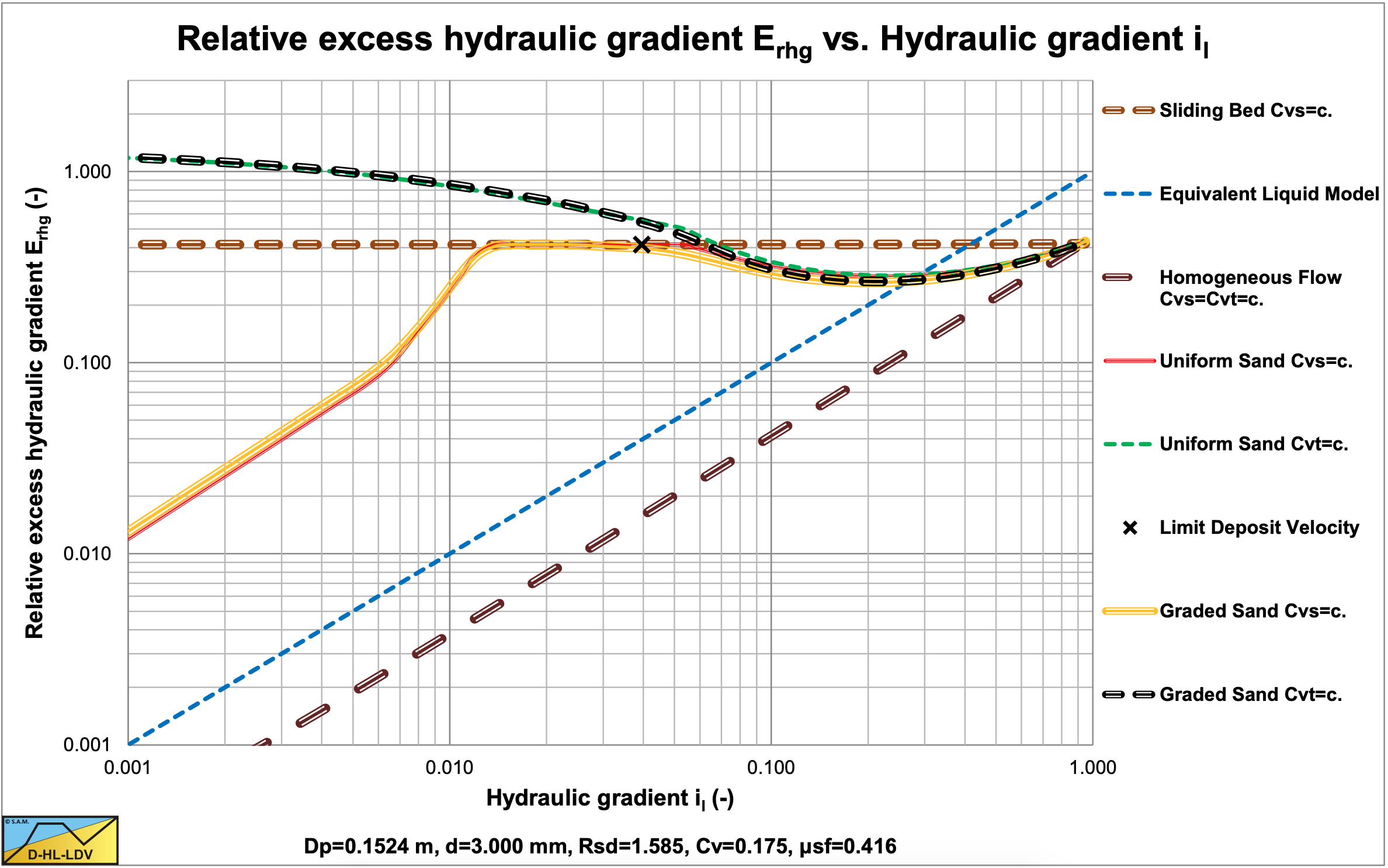
The values for A15 and A85 are 10.08. The graded relative excess hydraulic gradient curves are hardly higher than the uniform curves in the operational range of hydraulic gradients (0.01-0.1). In the homogeneous region, the curves are hardly higher than the theoretical homogeneous curve, because of the adjusted pseudo fluid properties. The fines diameter is d=0.067 mm and the percentage fines is 0.14% of the solids. The bed of the graded sand is slightly higher than the bed of the uniform sand.
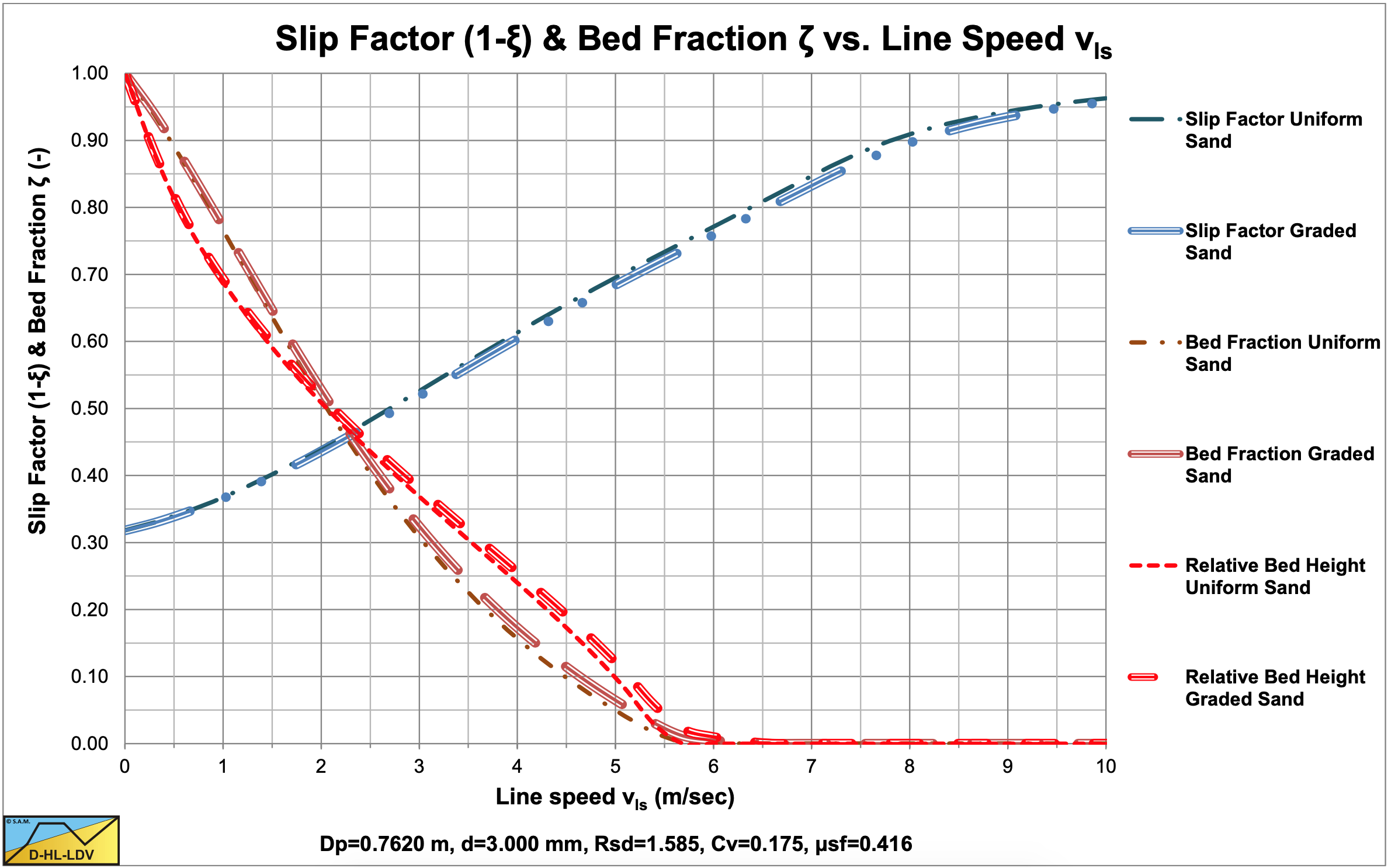
The values for A15 and A85 are 10.08. The graded relative excess hydraulic gradient curves are hardly higher than the uniform curves in the operational range of hydraulic gradients (0.01-0.1). In the homogeneous region, the curves are hardly higher than the theoretical homogeneous curve, because of the adjusted pseudo fluid properties. The fines diameter is d=0.109 mm and the percentage fines is 0.32% of the solids. The bed of the graded sand is slightly higher than the bed of the uniform sand. A larger pipe gives a larger fines diameter and a larger fines fraction.
7.13.10 Nomenclature PSD Influence
| \(\ \tilde{\mathrm{A}}_{\mathrm{b}}\) |
Bed fraction |
- |
| \(\ \tilde{\mathrm{A}}_{\mathrm{b}, \mathrm{i}}\) |
Bed fraction fraction i |
- |
|
Ax |
Constant in PSD function |
- |
|
A15 |
Constant in PSD function below d50 |
- |
|
A85 |
Constant in PSD function above d50 |
- |
|
Cvt |
Delivered (transport) volumetric concentration |
- |
|
Cvs |
Spatial volumetric concentration |
- |
|
Cvs,x |
Solids spatial concentration in pseudo liquid (fines) |
- |
|
Cvs,r |
Solids spatial concentration remaining after removing the fines from the PSD |
- |
|
Cvb |
Spatial volumetric concentration bed (1-n) |
- |
|
d |
Particle diameter |
m |
|
d15 |
Particle diameter with 15% passing |
m |
|
d50 |
Particle diameter with 50% passing |
m |
|
d85 |
Particle diameter with 85% passing |
m |
|
dlim |
Limiting particle diameter |
m |
|
dx |
Particle diameter |
m |
|
dy |
Particle diameter |
m |
|
Dp |
Pipe diameter |
m |
|
Erhg |
Relative excess hydraulic gradient in carrier liquid |
- |
|
Erhg,x |
Relative excess hydraulic gradient in pseudo liquid |
- |
|
fi |
Fraction i |
- |
|
fx |
PSD function |
- |
|
fy |
PSD function |
- |
|
g |
Gravitational constant 9.81 m/s2 |
m/s2 |
|
il |
Pure liquid hydraulic gradient |
m/m |
|
il,x |
Hydraulic gradient pseudo liquid |
m/m |
|
im |
Mixture hydraulic gradient |
m/m |
|
im,x |
Total mixture hydraulic gradient in pseudo liquid |
m/m |
|
im,x,i |
Mixture hydraulic gradient fraction i in pseudo liquid |
m/m |
|
n |
Number of fractions |
- |
|
p |
Probability distribution |
- |
|
Δpi |
Fraction i |
- |
|
Rsd |
Relative submerged density in carrier liquid |
- |
|
Rsd,x |
Relative submerged density in pseudo liquid |
- |
|
Stk |
Stokes number |
- |
|
X |
Fraction of sand in pseudo liquid |
- |
|
vls |
Line speed |
m/s |
|
vls,ldv |
Limit Deposit Velocity |
m/s |
|
vsl |
Slip velocity |
m/s |
|
vt |
Terminal settling velocity particle |
m/s |
|
wi |
Weigh factor fraction i |
- |
|
α15 |
d50 to d15 ratio |
- |
|
α85 |
d85 to d50 ratio |
- |
|
ρl |
Density liquid |
ton/m3 |
|
ρs |
Density solids |
ton/m3 |
|
ρx |
Density pseudo liquid |
ton/m3 |
|
ξ |
Slip ratio |
- |
|
ζ |
Bed fraction |
- |
|
ζi |
Bed fraction i |
- |
|
μsf |
Sliding friction coefficient |
- |
|
μl |
Dynamic viscosity carrier liquid |
Pa·s |
|
μx |
Dynamic viscosity pseudo liquid |
Pa·s |
| \(\ v_{\mathrm{l}}\) |
Kinematic viscosity carrier liquid |
m2/s |
| \(\ v_{\mathrm{x}}\) |
Kinematic viscosity pseudo liquid |
m2/s |