3.6: The Snow Plough Effect

3.6.1. The Normal and Friction Forces on the Shear Surface and Blade

On a cutter head, the blades can be divided into small elements, at which a two dimensional cutting process is considered. However, this is correct only when the cutting edge of this element is perpendicular to the direction of the velocity of the element. For most elements this will not be the case. The cutting edge and the absolute velocity of the cutting edge will not be perpendicular. This means the elements can be considered to be deviated with respect to the direction of the cutting velocity. A component of the cutting velocity perpendicular to the cutting edge and a component parallel to the cutting edge can be distinguished. This second component results in a deviation force on the blade element, due to the friction between the soil and the blade. This force is also the cause of the transverse movement of the soil, the snow plough effect.

To predict the deviation force and the direction of motion of the soil on the blade, the equilibrium equations of force will have to be solved in three directions. Since there are four unknowns, three forces and the direction of the velocity of the soil on the blade, one additional equation is required. This equation follows from an equilibrium equation of velocity between the velocity of grains in the shear zone and the velocity of grains on the blade. Since the four equations are partly non-linear and implicit, they have to be solved iteratively. The results of solving these equations have been compared with the results of laboratory tests on sand. The correlation between the two was very satisfactory, with respect to the magnitude of the forces and with respect to the direction of the forces and the flow of the soil on the blade.

Although the normal and friction forces as shown in Figure 3-14 are the basis for the calculation of the horizontal and vertical cutting forces, the approach used, requires the following equations to derive these forces by using equations (3-8) and (3-9). The index 1 points to the shear surface, while the index 2 points to the blade.

\[\ \mathrm{F}_{\mathrm{n} 1}=\mathrm{F}_{\mathrm{h}} \cdot \sin (\beta)-\mathrm{F}_{\mathrm{v}} \cdot \cos (\beta)\tag{3-47}\]

\[\ \mathrm{F}_{\mathrm{f} 1}=\mathrm{F}_{\mathrm{h}} \cdot \cos (\beta)+\mathrm{F}_{\mathrm{v}} \cdot \sin (\beta)\tag{3-48}\]

\[\ \mathrm{F}_{\mathrm{n} 2}=\mathrm{F}_{\mathrm{h}} \cdot \sin (\alpha)+\mathrm{F}_{\mathrm{v}} \cdot \cos (\alpha)\tag{3-49}\]

\[\ \mathrm{F_{f 2}=F_{h} \cdot \cos (\alpha)-F_{v} \cdot \sin (\alpha)}\tag{3-50}\]

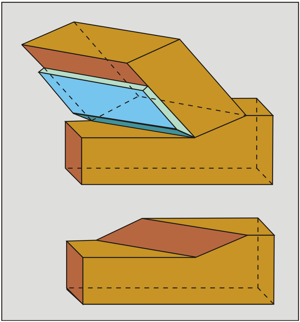
3.6.2. The 3D Cutting Theory

The previous paragraphs summarized the two-dimensional cutting theory. However, as stated in the introduction, in most cases the cutting process is not two-dimensional, because the drag velocity is not perpendicular to the cutting edge of the blade. Figure 3-16 shows this phenomenon. As with snow-ploughs, the soil will flow to one side while the blade is pushed to the opposite side. This will result in a third cutting force, the deviation force F_d. To determine this force, the flow direction of the soil has to be known. Figure 3-17 shows a possible flow direction.

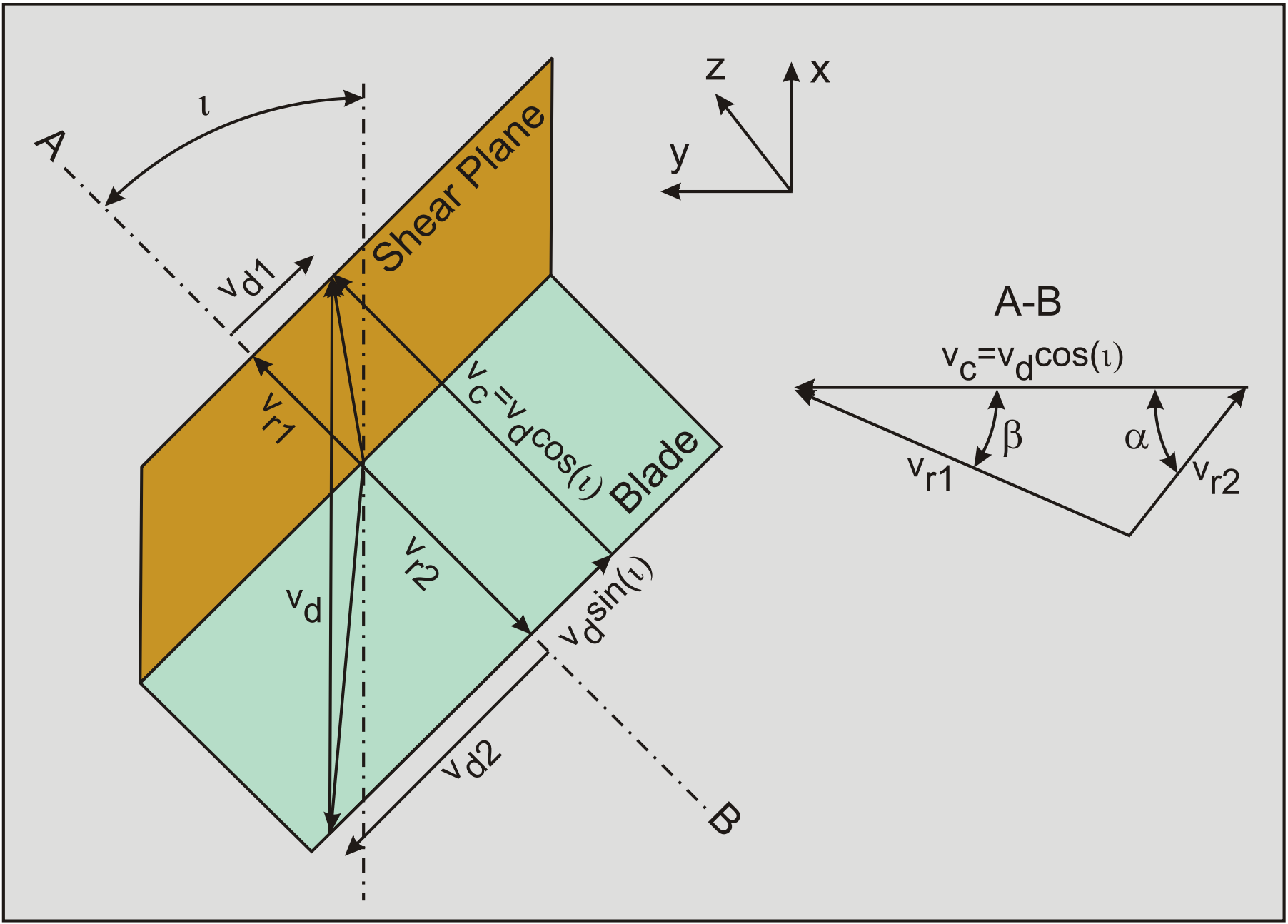
3.6.3. Velocity Conditions

For the velocity component perpendicular to the blade v_c, if the blade has a deviation angle \(\ \iota\) and a drag velocity v_d according to Figure 3-17, it yields:

\[\ \mathrm{v}_{\mathrm{c}}=\mathrm{v}_{\mathrm{d}} \cdot \cos (\mathrm{\iota})\tag{3-51}\]

The velocity of grains in the shear surface perpendicular to the cutting edge v_r1 is now:

\[\ \mathrm{v}_{\mathrm{r} 1}=\mathrm{v}_{\mathrm{c}} \cdot \frac{\sin (\alpha)}{\sin (\alpha+\beta)}\tag{3-52}\]

The relative velocity of grains with respect to the blade v_r2, perpendicular to the cutting edge is:

\[\ \mathrm{v}_{\mathrm{r} 2}=\mathrm{v}_{\mathrm{c}} \cdot \frac{\sin (\beta)}{\sin (\alpha+\beta)}\tag{3-53}\]

The grains will not only have a velocity perpendicular to the cutting edge, but also parallel to the cutting edge, the deviation velocity components v_d1 on the shear surface and v_d2 on the blade.

Figure 3-15: Urban winter service vehicle with snowplow (commons.wikimedia.org).

Figure 3-16: The 3D cutting process.

The velocity components of a grain in x, y and z direction can be determined by considering the absolute velocity of grains in the shear surface, this leads to:

\[\ \overrightarrow{\mathrm{v}}_{\mathrm{r} 2}+\overrightarrow{\mathrm{v}}_{\mathrm{d} 2}+\overrightarrow{\mathrm{v}}_{\mathrm{d}}=\overrightarrow{\mathrm{v}}_{\mathrm{r} 1}+\overrightarrow{\mathrm{v}}_{\mathrm{d} 1}\tag{3-54}\]

\[\ \mathrm{v}_{\mathrm{x} 1}=\mathrm{v}_{\mathrm{r} 1} \cdot \cos (\beta) \cdot \cos (\mathfrak{\iota})+\mathrm{v}_{\mathrm{d} 1} \cdot \sin (\iota)\tag{3-55}\]

\[\ \mathrm{v}_{\mathrm{y} 1}=\mathrm{v}_{\mathrm{r} 1} \cdot \cos (\beta) \cdot \sin (\mathrm{\iota})-\mathrm{v}_{\mathrm{d} 1} \cdot \cos (\mathrm{\iota})\tag{3-56}\]

\[\ \mathrm{v}_{\mathrm{z 1}}=\mathrm{v}_{\mathrm{r} \mathrm{1}} \cdot \sin (\beta)\tag{3-57}\]

Figure 3-17: Velocity conditions.

Figure 3-18: Force directions.

The velocity components of a grain can also be determined by a summation of the drag velocity of the blade and the relative velocity between the grains and the blade, this gives:

\[\ \mathrm{v}_{\mathrm{x} 2}=\mathrm{v}_{\mathrm{d}}-\mathrm{v}_{\mathrm{r} 2} \cdot \cos (\alpha) \cdot \cos (\iota)-\mathrm{v}_{\mathrm{d} 2} \cdot \sin (\mathfrak{\iota})\tag{3-58}\]

\[\ \mathrm{v}_{\mathrm{y} 2}=-\mathrm{v}_{\mathrm{r} 2} \cdot \cos (\alpha) \cdot \sin ({\iota})+\mathrm{v}_{\mathrm{d} 2} \cdot \cos (\iota)\tag{3-59}\]

\[\ \mathrm{v}_{\mathrm{z} 2}=\mathrm{v}_{\mathrm{r} 2} \cdot \sin (\alpha)\tag{3-60}\]

Since both approaches will have to give the same resulting velocity components, the following condition for the transverse velocity components can be derived:

\[\ \mathrm{v}_{\mathrm{x} 1}=\mathrm{v}_{\mathrm{x} 2} \Longrightarrow \mathrm{v}_{\mathrm{d} 1}+\mathrm{v}_{\mathrm{d} 2}=\mathrm{v}_{\mathrm{d}} \cdot \sin (\mathfrak{\iota})\tag{3-61}\]

\[\ \mathrm{v}_{\mathrm{y} 1}=\mathrm{v}_{\mathrm{y} 2} \Longrightarrow \mathrm{v}_{\mathrm{d} 1}+\mathrm{v}_{\mathrm{d} 2}=\mathrm{v}_{\mathrm{d}} \cdot \sin (\mathrm{\iota})\tag{3-62}\]

\[\ \mathrm{v}_{\mathrm{z} \mathrm{1}}=\mathrm{v}_{\mathrm{z} \mathrm{2}}\tag{3-63}\]

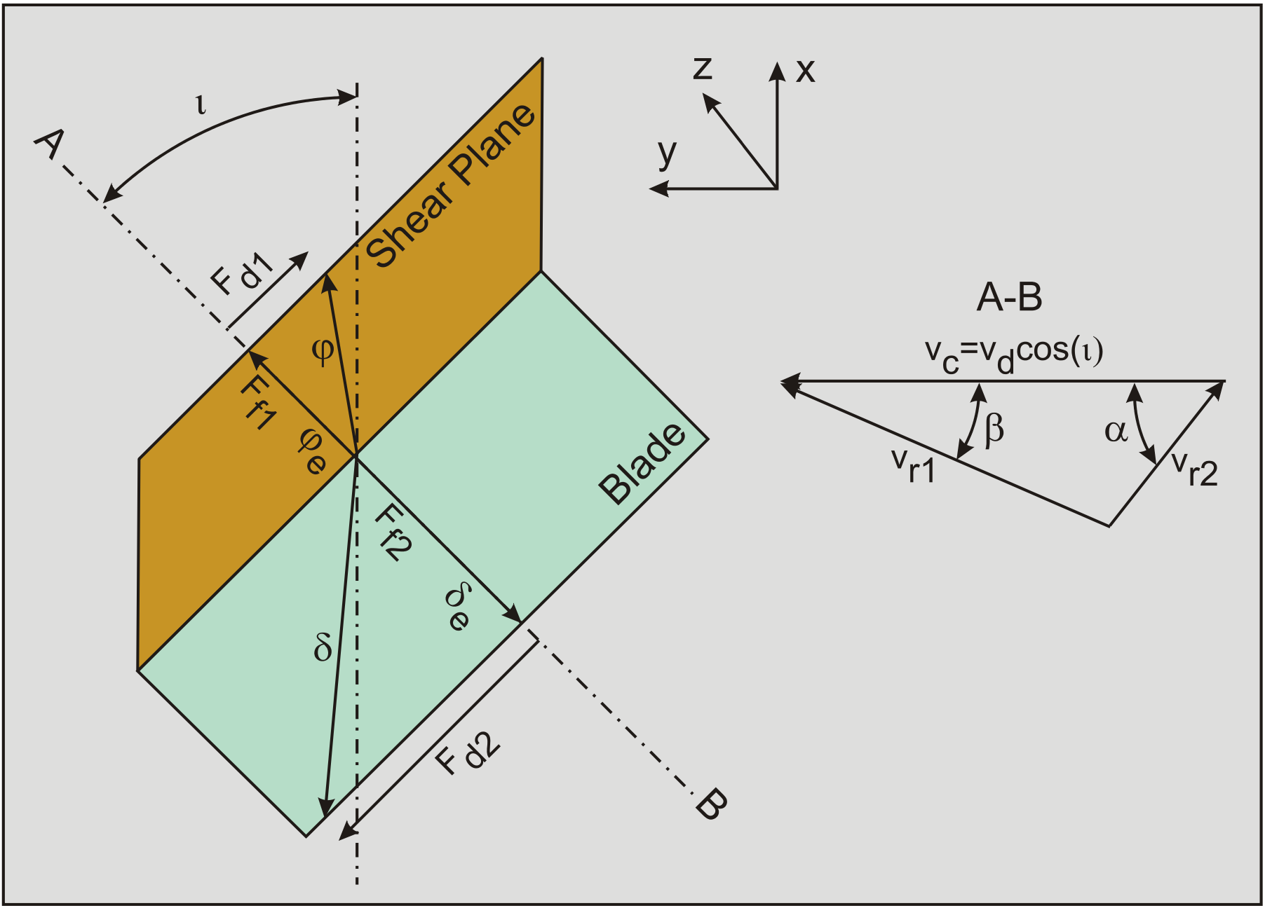
3.6.4. The Deviation Force

Since a friction force always has a direction matching the direction of the relative velocity between two bodies, the fact that a deviation velocity exists on the shear surface and on the blade, implies that also deviation forces must exist. To match the direction of the relative velocities, the following equations can be derived for the deviation force on the shear surface and on the blade (Figure 3-18):

\[\ \mathrm{F}_{\mathrm{d} 1}=\mathrm{F}_{\mathrm{f} 1} \cdot \frac{\mathrm{v}_{\mathrm{d} 1}}{\mathrm{v}_{\mathrm{r} 1}}\tag{3-64}\]

\[\ \mathrm{F}_{\mathrm{d} 2}=\mathrm{F}_{\mathrm{f} 2} \cdot \frac{\mathrm{v}_{\mathrm{d} 2}}{\mathrm{v}_{\mathrm{r} 2}}\tag{3-65}\]

Since perpendicular to the cutting edge, an equilibrium of forces exists, the two deviation forces must be equal in magnitude and have opposite directions.

\[\ \mathrm{F}_{\mathrm{d} \mathrm{1}}=\left|\mathrm{F}_{\mathrm{d} 2}\right|\tag{3-66}\]

By substituting equations (3-64) and (3-65) in equation (3-66) and then substituting equations (3-48) and (3-50) for the friction forces and equations (3-52) and (3-53) for the relative velocities, the following equation can be derived, giving a second relation between the two deviation velocities:    

\[\ \lambda=\frac{\mathrm{v}_{\mathrm{d} 1}}{\mathrm{v}_{\mathrm{d} 2}}=\left(\frac{\mathrm{F}_{\mathrm{f} 2}}{\mathrm{F}_{\mathrm{f} 1}}\right) \cdot\left(\frac{\mathrm{v}_{\mathrm{r} 1}}{\mathrm{v}_{\mathrm{r} 2}}\right)=\left(\frac{\mathrm{F}_{\mathrm{h}} \cdot \cos (\alpha)-\mathrm{F}_{\mathrm{v}} \cdot \sin (\alpha)}{\mathrm{F}_{\mathrm{h}} \cdot \cos (\beta)+\mathrm{F}_{\mathrm{v}} \cdot \sin (\beta)}\right) \cdot\left(\frac{\sin (\alpha)}{\sin (\beta)}\right)\tag{3-67}\]

To determine F_h and F_v perpendicular to the cutting edge, the angle of internal friction φ_e and the external friction angle δ_e mobilized perpendicular to the cutting edge, have to be determined by using the ratio of the transverse velocity and the relative velocity, according to:

\[\ \tan \left(\varphi_{\mathrm{e}}\right)=\tan (\varphi) \cdot \cos \left(\operatorname{atn}\left(\frac{\mathrm{v}_{\mathrm{d} 1}}{\mathrm{v}_{\mathrm{r} 1}}\right)\right)\tag{3-68}\]

\[\ \tan \left(\delta_{\mathrm{e}}\right)=\tan (\delta) \cdot \cos \left(\operatorname{atn}\left(\frac{\mathrm{v}_{\mathrm{d} 2}}{\mathrm{v}_{\mathrm{r}} 2}\right)\right)\tag{3-69}\]

For the cohesion c and the adhesion a this gives:

\[\ \mathrm{c}_{\mathrm{e}}=\mathrm{c \cdot cos ( \mathrm { a t n } ( \frac { \mathrm { v } _ { \mathrm { d } 1 } } { \mathrm { v } _ { \mathrm { r } 1 } } ) )}\tag{3-70}\]

\[\ \mathrm{a}_{\mathrm{e}}=\mathrm{a} \cdot \cos \left(\operatorname{atn}\left(\frac{\mathrm{v}_{\mathrm{d} 2}}{\mathrm{v}_{\mathrm{r} 2}}\right)\right)\tag{3-71}\]

3.6.5. The Resulting Cutting Forces

The resulting cutting forces in x, y and z direction can be determined once the deviation velocity components are known. However, it can be seen that the second velocity condition equation (3-67) requires the horizontal and vertical cutting forces perpendicular to the cutting edge, while these forces can only be determined if the mobilized internal and external friction angles and the mobilized cohesion and adhesion (equations (3-68), (3-69), (3-70) and (3-71)) are known. This creates an implicit set of equations that will have to be solved by means of an iteration process. For the cutting forces on the blade the following equation can be derived:

\[\ \mathrm{F}_{\mathrm{x} 2}=\mathrm{F}_{\mathrm{h}} \cdot \cos (\mathrm{\iota})+\mathrm{F}_{\mathrm{d} 2} \cdot \sin (\mathrm{\iota})\tag{3-72}\]

\[\ \mathrm{F}_{\mathrm{y} 2}=\mathrm{F}_{\mathrm{h}} \cdot \sin ({\iota})-\mathrm{F}_{\mathrm{d} 2} \cdot \cos (\iota)\tag{3-73}\]

\[\ \mathrm{F}_{\mathrm{z} 2}=\mathrm{F}_{\mathrm{v}}\tag{3-74}\]

The problem of the model being implicit can be solved in the following way:

A new variable λ is introduced in such a way that:

\[\ \mathrm{v_{d 1}=\frac{\lambda}{1+\lambda} \cdot v_{d} \cdot \sin (\iota)}\tag{3-75}\]

\[\ \mathrm{v}_{\mathrm{d} 2}=\frac{\mathrm{1}}{\mathrm{1}+\lambda} \cdot \mathrm{v}_{\mathrm{d}} \cdot \sin (\iota)\tag{3-76}\]

This satisfies the condition from equations (3-61) and (3-62) for the sum of these 2 velocities:

\[\ \mathrm{v}_{\mathrm{d} 1}+\mathrm{v}_{\mathrm{d} 2}=\mathrm{v}_{\mathrm{d}} \cdot \sin (\iota)\tag{3-77}\]

The procedure starts with a starting value for λ=1. Based on the velocities found with equations (3-75), (3-76), (3-52) and (3-53), the mobilized internal φ_e and external δ_e friction angles and the cohesion c_e and adhesion a_e can be determined using the equations (3-68), (3-69), (3-70) and (3-71). Once these are known, the horizontal F_h and vertical F_v cutting forces in the plane perpendicular to the cutting edge can be determined with equations (3-8) and (3-9). With the equations (3-48), (3-50), (3-64) and (3-65) the friction and deviation forces on the blade and the shear plane can be determined. Now with equation (3-67) the value of the variable λ can be determined and if the starting value is correct, this value should be found. In general this will not be the case after one iteration. But repeating this procedure 3 or 4 times should give enough accuracy.