2: Mathematical Tools
- Page ID
- 77050

\( \newcommand{\vecs}[1]{\overset { \scriptstyle \rightharpoonup} {\mathbf{#1}} } \)
\( \newcommand{\vecd}[1]{\overset{-\!-\!\rightharpoonup}{\vphantom{a}\smash {#1}}} \)
\( \newcommand{\dsum}{\displaystyle\sum\limits} \)
\( \newcommand{\dint}{\displaystyle\int\limits} \)
\( \newcommand{\dlim}{\displaystyle\lim\limits} \)
\( \newcommand{\id}{\mathrm{id}}\) \( \newcommand{\Span}{\mathrm{span}}\)
( \newcommand{\kernel}{\mathrm{null}\,}\) \( \newcommand{\range}{\mathrm{range}\,}\)
\( \newcommand{\RealPart}{\mathrm{Re}}\) \( \newcommand{\ImaginaryPart}{\mathrm{Im}}\)
\( \newcommand{\Argument}{\mathrm{Arg}}\) \( \newcommand{\norm}[1]{\| #1 \|}\)
\( \newcommand{\inner}[2]{\langle #1, #2 \rangle}\)
\( \newcommand{\Span}{\mathrm{span}}\)
\( \newcommand{\id}{\mathrm{id}}\)
\( \newcommand{\Span}{\mathrm{span}}\)
\( \newcommand{\kernel}{\mathrm{null}\,}\)
\( \newcommand{\range}{\mathrm{range}\,}\)
\( \newcommand{\RealPart}{\mathrm{Re}}\)
\( \newcommand{\ImaginaryPart}{\mathrm{Im}}\)
\( \newcommand{\Argument}{\mathrm{Arg}}\)
\( \newcommand{\norm}[1]{\| #1 \|}\)
\( \newcommand{\inner}[2]{\langle #1, #2 \rangle}\)
\( \newcommand{\Span}{\mathrm{span}}\) \( \newcommand{\AA}{\unicode[.8,0]{x212B}}\)
\( \newcommand{\vectorA}[1]{\vec{#1}} % arrow\)
\( \newcommand{\vectorAt}[1]{\vec{\text{#1}}} % arrow\)
\( \newcommand{\vectorB}[1]{\overset { \scriptstyle \rightharpoonup} {\mathbf{#1}} } \)
\( \newcommand{\vectorC}[1]{\textbf{#1}} \)
\( \newcommand{\vectorD}[1]{\overrightarrow{#1}} \)
\( \newcommand{\vectorDt}[1]{\overrightarrow{\text{#1}}} \)
\( \newcommand{\vectE}[1]{\overset{-\!-\!\rightharpoonup}{\vphantom{a}\smash{\mathbf {#1}}}} \)
\( \newcommand{\vecs}[1]{\overset { \scriptstyle \rightharpoonup} {\mathbf{#1}} } \)
\(\newcommand{\longvect}{\overrightarrow}\)
\( \newcommand{\vecd}[1]{\overset{-\!-\!\rightharpoonup}{\vphantom{a}\smash {#1}}} \)
\(\newcommand{\avec}{\mathbf a}\) \(\newcommand{\bvec}{\mathbf b}\) \(\newcommand{\cvec}{\mathbf c}\) \(\newcommand{\dvec}{\mathbf d}\) \(\newcommand{\dtil}{\widetilde{\mathbf d}}\) \(\newcommand{\evec}{\mathbf e}\) \(\newcommand{\fvec}{\mathbf f}\) \(\newcommand{\nvec}{\mathbf n}\) \(\newcommand{\pvec}{\mathbf p}\) \(\newcommand{\qvec}{\mathbf q}\) \(\newcommand{\svec}{\mathbf s}\) \(\newcommand{\tvec}{\mathbf t}\) \(\newcommand{\uvec}{\mathbf u}\) \(\newcommand{\vvec}{\mathbf v}\) \(\newcommand{\wvec}{\mathbf w}\) \(\newcommand{\xvec}{\mathbf x}\) \(\newcommand{\yvec}{\mathbf y}\) \(\newcommand{\zvec}{\mathbf z}\) \(\newcommand{\rvec}{\mathbf r}\) \(\newcommand{\mvec}{\mathbf m}\) \(\newcommand{\zerovec}{\mathbf 0}\) \(\newcommand{\onevec}{\mathbf 1}\) \(\newcommand{\real}{\mathbb R}\) \(\newcommand{\twovec}[2]{\left[\begin{array}{r}#1 \\ #2 \end{array}\right]}\) \(\newcommand{\ctwovec}[2]{\left[\begin{array}{c}#1 \\ #2 \end{array}\right]}\) \(\newcommand{\threevec}[3]{\left[\begin{array}{r}#1 \\ #2 \\ #3 \end{array}\right]}\) \(\newcommand{\cthreevec}[3]{\left[\begin{array}{c}#1 \\ #2 \\ #3 \end{array}\right]}\) \(\newcommand{\fourvec}[4]{\left[\begin{array}{r}#1 \\ #2 \\ #3 \\ #4 \end{array}\right]}\) \(\newcommand{\cfourvec}[4]{\left[\begin{array}{c}#1 \\ #2 \\ #3 \\ #4 \end{array}\right]}\) \(\newcommand{\fivevec}[5]{\left[\begin{array}{r}#1 \\ #2 \\ #3 \\ #4 \\ #5 \\ \end{array}\right]}\) \(\newcommand{\cfivevec}[5]{\left[\begin{array}{c}#1 \\ #2 \\ #3 \\ #4 \\ #5 \\ \end{array}\right]}\) \(\newcommand{\mattwo}[4]{\left[\begin{array}{rr}#1 \amp #2 \\ #3 \amp #4 \\ \end{array}\right]}\) \(\newcommand{\laspan}[1]{\text{Span}\{#1\}}\) \(\newcommand{\bcal}{\cal B}\) \(\newcommand{\ccal}{\cal C}\) \(\newcommand{\scal}{\cal S}\) \(\newcommand{\wcal}{\cal W}\) \(\newcommand{\ecal}{\cal E}\) \(\newcommand{\coords}[2]{\left\{#1\right\}_{#2}}\) \(\newcommand{\gray}[1]{\color{gray}{#1}}\) \(\newcommand{\lgray}[1]{\color{lightgray}{#1}}\) \(\newcommand{\rank}{\operatorname{rank}}\) \(\newcommand{\row}{\text{Row}}\) \(\newcommand{\col}{\text{Col}}\) \(\renewcommand{\row}{\text{Row}}\) \(\newcommand{\nul}{\text{Nul}}\) \(\newcommand{\var}{\text{Var}}\) \(\newcommand{\corr}{\text{corr}}\) \(\newcommand{\len}[1]{\left|#1\right|}\) \(\newcommand{\bbar}{\overline{\bvec}}\) \(\newcommand{\bhat}{\widehat{\bvec}}\) \(\newcommand{\bperp}{\bvec^\perp}\) \(\newcommand{\xhat}{\widehat{\xvec}}\) \(\newcommand{\vhat}{\widehat{\vvec}}\) \(\newcommand{\uhat}{\widehat{\uvec}}\) \(\newcommand{\what}{\widehat{\wvec}}\) \(\newcommand{\Sighat}{\widehat{\Sigma}}\) \(\newcommand{\lt}{<}\) \(\newcommand{\gt}{>}\) \(\newcommand{\amp}{&}\) \(\definecolor{fillinmathshade}{gray}{0.9}\)In this chapter we introduce a few mathematical tools that we will use in formulating some of the analysis of fluid flow problems for both inviscid and viscous flows. We introduce the use of tensor notation which is widely used in expressing fluid mechanics governing equations. We also show some mathematical manipulations that will help to provide some physical insight into the governing equations.
Tensor Notation
Most students are very familiar with vector notation (or Gibbs notation) for describing (usually) three component vectors in fluid mechanics. Vector notation implies the existence of components of the vector. A scalar, as is known is fully described by a single number, its magnitude. Of course a vector quantity may have more than three components in general, but here we are using vectors to describe components in three dimensional space. Each component may be a function of both space and time, and as such the entire vector is a function of space and time. The number of components in the vector is determined by the “dimensionality” of the vector. For instance a velocity field may only have two orthogonal directions, say (x,y), and as such the flow becomes two dimensional — the assumption is that there is no velocity variation in the third, z, direction. We can think of the three components as a set of three independent variables that the variable in question is a function of.
Tensor notation is an alternative approach and is a very powerful way of expressing any dimensional vector, as well as what are known as higher order tensors — variables that have several sets of independent variables to be considered. We say that a scalar is a zero order tensor and a vector is a first order tensor, such as velocity. An example of a second order tensor is stress. It requires two sets of indices to define its local value. A third order tensor requires a set of three indices to be fully defined. In our three dimensional world then, a first order tensor has three components. A second order tensor has nine components, determined by the possible combinations of the three elements within each set of indices. To make this clear note that for some vector V in three dimensions:
\[\textbf{V}= u\textbf{i}+v\textbf{j}+w\textbf{k }={u{}_{i}}\]
Where u,v, and w are the values of the three components each a function of (x,y,z), \(\textbf{i},\textbf{j}\) and \(\textbf{k}\) are the unit vectors associated with x,y and z coordinates respectively and \(u{}_{i}\) is tensor notation for a vector \(V\). The tensor representation uses a subscript which can have three possible values, each representing one of the three components the vector, or \(u{}_{1} = u, u{}_{2}\) = v and \(u{}_{3} = w\). Each component is denoted by a particular subscript that is defined based on the numerical value of the index. Here index number “1” is representative of the x coordinate, etc. But this is not limited to Cartesian coordinates. For example subscripts 1, 2 and 3 could represent r, \(\theta\) and z in cylindrical coordinates.
Also, we can define a stress tensor as:
\[\tau_{ij}\]
and the number of possible combinations of the subscripts i,j are nine. Do not confuse these subscripts with the unit vectors since they can take on one of the possible three directions. For fluid flow problems we will define the stress tensor and use it to arrive at our conservation of momentum equation. A third order tensor could be written as \(T{}_{ijk}\) and it would have 27 elements (3x3x3). As stated above, a single subscript denotes a vector and has 3 possible values, one for each coordinate.
It is possible to write all of our vector equations using tensors instead of the vector notation. This has some advantages and is used widely in fluid mechanics. Table 2.1 illustrates a number of examples of the equivalence of vector and tensor notation. A few of these are worth discussing and we will be using them as we write out the various equations that we will be formulating and using. It is suggested that you examine this notation and look at the various operators listed.
Operations among vectors carry with them some special consideration and rules. The gradient operator is \(\mathrm{\nabla }\) in vector notation. If the quantity of interest is the gradient of scalar “a”, written as \(\mathrm{\nabla }\mathrm{a\ }\), then this operation results in a vector whose components are partial derivatives in each of the three coordinates, \(\frac{\partial a}{\partial x}\) is the x component, etc. In tensor operation this is expressed as \(\frac{\partial a}{\partial x_i}\) which is a vector whose components correspond to each of the three possible values of the index “\({i}\)”. If the gradient is being taken of a vector, say \({u{}_{j}}\), the the resulting gradient expression is a second order tensor with the two indices, \({i }\) for the partial derivatives and \(\textit{j}\) for the vector quantity \({u{}_{j}}\). This is then written as \(\frac{\partial u_j}{\partial x_i}\). Notice that the gradient operator index comes first since it operates on the vector \({u{}_{j}}\). There are nine combinations of \({i,j}\) for this second order tensor. We will see this tensor in our discussions of viscous flows and vorticity.
| Examples of Vector VS Tensor Notation | ||
|---|---|---|
| Quality | Vector Notation | Tensor Notation |
| Scalar | a | a |
| Vector | \(\bar{a}\) | \(a_i\) |
| 2nd order tensor | \(\overline{\overline{a}}\)
|
\(a_{ij}\) |
| dot product (scalar) | \(\bar{a}\cdot\bar{b}\) | \(a_{i} b_{i}\) |
| cross product (vector) | \(\bar{a}\times\bar{b}\) | \(\varepsilon_{ijk}a_{j}b_{k}\) |
| del operator (vector) | \(\bigtriangledown\) | \(\frac{\partial}{\partial x_i}\) |
| gradient (vector; tensor) | \(\bigtriangledown a;\bigtriangledown\bar{a}\) | \(\frac{\partial{a}}{\partial {x_{i}}};\frac{\partial{a_{i}}}{\partial{x_{j}}}\) |
| divergence (scalar) | \(\bigtriangledown\cdot\bar{a}\) | \(\frac{\partial{a_{i}}}{\partial{x_{i}}}\) |
| curl (vector) | \(\bigtriangledown\times\bar{a}\) | \(\varepsilon_{ijk}\frac{\partial{a_k}}{\partial{x_j}}\) |
| Laplace operator (scalar) | \(\bigtriangledown^2\) | \(\frac{\partial^2}{\partial{x_i}\partial{x_i}}\) |
| divergence of a 2nd order tensor | \(\bigtriangledown\cdot \overline{\overline{a}}\) | \(\frac{\partial{a_y}}{\partial{x_i}}(vector)\) |
| dot product: vector & del | \(\bar{a}\cdot\bigtriangledown\) | \(a_j\frac{\partial}{\partial{x_j}}(scalar)\) |
| dot product: vector & gradient | \(\bar{a}\cdot\bigtriangledown\bar{b}\) | \(a_j\frac{\partial{b_i}}{\partial{x_j}}(vector)\) |
| Material Derivative | \(\frac{\partial}{\partial{t}}+\bar{u}\cdot\bigtriangledown or \frac{D}{Dt}\) | |
| Vorticity: (pseudovector) | \(\omega_k=\bigtriangledown \text{x}\bar{u}=\left (\frac{\partial{u_i}} {\partial{u_j}}-\frac{\partial{x_j}}{\partial{x_i}} \right )=\varepsilon_{ijk}\frac{\partial {u_k}}{\partial{x_j}}\) | |
| Rate of strain tensor: (2nd order tensor) | \(\frac{1}{2}\left (\frac{\partial{u_i}} {\partial{u_j}}+\frac{\partial{u_j}}{\partial{u_i}} \right )\) |
Consider now the divergence operation, in vector notation written as \(\mathrm{\nabla }\mathrm{\cdot }\mathrm{V}\). This operation is the dot, or scalar, product between the vector operator \(\mathrm{\nabla }\) and vector V. The result is a scalar. The tensor notation for this operation is \(\frac{\partial u_i}{\partial x_i}\) where the indices for the vector \({u{}_{i}}\) are the same as the index for the partial derivative operator. This implies that the same component of each vector, \(\mathrm{\nabla }\) and V, should be used simultaneously. The rule in tensor notation then is to add all of these component operations to result in one final scalar. This becomes for the three coordinates, \(x{}_{1}, x{}_{2}\) and \(x{}_{3}{}_{,\ }\) which in Cartesian coordinates are x, y and z: \(\frac{\partial u_i}{\partial x_i}=\frac{\partial u_1}{\partial x_1}+\frac{\partial u_2}{\partial x_2}+\frac{\partial u_3\ }{\partial x_3}\ =\ \frac{\partial u}{\partial x}+\frac{\partial v}{\partial y}+\frac{\partial w}{\partial z}\)
The result is a scalar formed from the sum of each of the partial derivatives. As is apparent from this equation, when a term has a “repeated” index (such as the index “\({i}\)” in the above equation for both u and x) then the rule is to sum over all values of the index. This applies to a particular term in an equation.As an additional example consider the term \(\frac{\partial a_{ij}}{\partial x_i}\)in this case the index “\({i}\)” is repeated and j is left as a “free index” (which could take on any of the possible three coordinate values.) Consequently this expression is a vector, with one free index, whose components are represented by the value of “\({j}\)”.There is also an operator, \({\varepsilon }_{ijk}\). This is given the name “permutation operator”. Notice in Table 2.1 this is listed as used in the cross product and curl operation (the curl is the cross product of the vector operator \(\mathrm{\nabla }\), which in tensor notation is written as \(\frac{\partial }{\partial x_j}\), and the vector \({u{}_{k}})\). The permutation operator definition results in the cross product between two vectors. For this each of the indices can take on three different values, and there are 27 different possible combinations. The rules associated with the different values are as follows:
- if any of the three indices have the same value then \({\varepsilon }_{ijk}{}_{\ }= 0\)
- if the order of the indices is cyclic (1,2,3 or 2,3,1 or 3,1,2) then \({\varepsilon }_{ijk} ={\ }1\)
- if the order of the indices is anti-cyclic (1,3,2 or 2,1,3 or 3,2,1) then \({\varepsilon }_{ijk\ }={ }_{\ }-1\)
\[a_j\times b_k={\varepsilon }_{ijk}a_jb_k=\left(a_2b_3-a_3b_2\right)\boldsymbol{i}+\left(a_3b_1-a_1b_3\right)\boldsymbol{j}\boldsymbol{+}\left(a_1b_2-a_2b_1\right)\boldsymbol{k}\]
The reader should perform this operation for the curl of a vector where \(a_i\) is replaced by \(\frac{\partial }{\partial x_j}\) and \({b{}_{k}}\) is replaced by \({u{}_{k}}\)
There is another often used operator in tensor notation called the Kronecker delta, \({\delta}_{ij}\). The rule used is that when \({i=j}\) the value of \({\delta}_{ij}\) is one, otherwise it is set equal to zero, that is:
\[{\delta }_{ij}=1\ for\ i=j\\\]
\[{\delta }_{ij}=0\ for\ i\neq j\\\]
This comes in handy when one wants to include terms where there may be a nonzero value only when \({i=j}\). We will see this in our expression in the Navier-Stokes equation for the pressure contribution to the total force on a fluid element. For example suppose we want to include a gradient of a scalar, \({S}\), as \(\frac{\partial S}{\partial x_j}\) in an equation, note that this is a vector quantity. However, if we are evaluating different components of the gradient we only want to include those components that align with the vector component “\({i}\)”, then we would write this term \(\frac{\partial S}{\partial x_j}
Callstack:
    at (Bookshelves/Civil_Engineering/Intermediate_Fluid_Mechanics_(Liburdy)/02:_Mathematical_Tools), /content/body/div[1]/p[17]/span, line 1, column 1
Gradient, Divergence and Curl Operators
The gradient is a vector operator that for instance, when operated on a scalar produces a vector. It takes the partial derivative with respect to each component of the coordinate system. It is denoted as \(\bigtriangledown\) and can be expressed in Cartesian coordinates as:
\[\bigtriangledown ( ) = \frac {\partial ( )} {\partial x}i + \frac {\partial ( )} {\partial y}j + \frac {\partial ( )} {\partial z} k\]
Where a scalar of a vector or tensor could be inserted into the parenthesis. A gradient of a vector then has 9 components, where you take x,y,z derivatives of each of the three vector components. This would form the secord order tensor:
\[\bigtriangledown V =\begin{bmatrix} \frac{\partial u}{\partial x}&\frac{\partial u}{\partial y} &\frac{\partial u}{\partial z} \\ \frac{\partial v}{\partial x}&\frac{\partial v}{\partial y} &\frac{\partial v}{\partial z} \\ \frac{\partial w}{\partial x}&\frac{\partial w}{\partial y} &\frac{\partial w}{\partial z} \end{bmatrix}\]
If one takes the dot product of \(\bigtriangledown\) with a vector we get the divergence of that vector which is a scaler:
\[\bigtriangledown\cdot V = \frac {\partial u} {\partial x} + \frac {\partial v} {\partial y} + \frac {\partial w} {\partial z}\]
Note that the divergence of the second order tensor yields a vector, such as \(\bigtriangledown\cdot\bigtriangledown{V}\). The x component of this vector is:
\[\bigtriangledown\cdot{\bigtriangledown u} = \left ( \frac{\partial^2u}{\partial{x^2}}+\frac{\partial^2u}{\partial{y^2}}+\frac{\partial^2u}{\partial{z^2}} \right )i\]
The y and z components should be apparent where the x component of velocity is replaced by the y and z components of velocity in the numerators for the y and z components of the resultant vector.
Vector Identities
Vector Identity
Below are shown a few vector identities that are used in fluid mechanics in the manipulation of the governing equations of motion. A,B are vectors, \(phi\), is a scalar.
\[\bigtriangledown\left ( A \cdot B \right ) = \left (A\cdot\bigtriangledown \right )B+\left ( B\cdot\bigtriangledown \right )A+A\cdot\left ( \bigtriangledown\cdot B \right )+ B \cdot\left ( \bigtriangledown\cdot A \right ) = A\bigtriangledown{B} + B\bigtriangledown{A}\]
\[\frac{1}{2}\bigtriangledown\left ( A\cdot{A} \right )=\left ( A\cdot\bigtriangledown \right )A+A\cdot\left ( \bigtriangledown + A \right ) = A\bigtriangledown{A}\]
\[\bigtriangledown\cdot\left ( \bigtriangledown\phi \right )=0\]
\[\bigtriangledown\cdot\left ( \bigtriangledown\cdot{A} \right )=0\]
\[\bigtriangledown^2\phi=\bigtriangledown\cdot\left ( \bigtriangledown\phi \right )\]
\[\bigtriangledown\cdot\left ( \bigtriangledown\cdot A \right )=\bigtriangledown\left ( \bigtriangledown\cdot A \right )-\bigtriangledown^2A\]
Divergence Theorem: What is the name of this symbol? \(B\cdot{d}A = \int\int\int\left ( \bigtriangledown\cdot B \right )d V\) (where \(dA\) is an elemental area around the boundary of volume \(V\))
Stokes’ Theorem: \(\oint B\cdot d l = \int \int \left ( \bigtriangledown\cdot B \right )\cdot d A\) (where \(dl\) is an element of the line integral around the boundary of area \(A\)).
There are a number of vector identities and manipulations that are very useful in fluid mechanics. We list a few of these here for future reference. Unless stated otherwise these are valid for any vector quantity, \(V\).
Material Derivative
The material derivative is a shorthand notation expressing the rate change of some property or parameter, which could be a scalar or a tensor, such as temperature, pressure or momentum (mass times velocity). This time derivative is based on a Lagrangian frame of reference of a fixed mass of fluid. So in a sense one is following a fixed mass of fluid and describing how the given property changes. Since the fluid mass can move we say that the fixed mass depends on both space and time. For example if we pick the scalar pressure, \({P}\), and say that our fixed mass has a pressure that is a function of space and time using Cartesian coordinates we have for the variable pressure:
\[{P }= {f}(x,y,z,t\textit{)}\]
Then if we want its time rate of change for a fixed mass at a given time we use the notation that \({DP}\) is the change of quantity \({P}\) and  is its change over time accounting for changes in both space and time (note we apply the chain rule for each of the possible coordinate directions:
\[\frac{DP}{Dt}=\frac{\partial P}{\partial t}+\frac{\partial P}{\partial x}\frac{dx}{dt}+\frac{\partial P}{\partial y}\frac{dy}{dt}+\frac{\partial P}{\partial z}\frac{dz}{dt}\]
Noting that \(\frac{dx}{dt}=u\) and similarly for each coordinate direction, the equation becomes:
\[\frac{DP}{Dt}=\frac{\partial P}{\partial t}+u\frac{\partial P}{\partial x}+v\frac{\partial P}{\partial y}+w\frac{\partial P}{\partial z}\label{2.1} \]
Things to pay attention to in this equation are (i) the velocity components \({u,v}\) and \({w}\) are not vector quantities, but components of the velocity vector, V; (ii) the time variation is specified by the first term and is evaluated at a particular point in space (as are all of the other terms) but all other terms may in fact be time dependent; this equation is valid for scalars or tensors, and the tensor sense is determined by the quantity being evaluated (in Equation (2.1) it is a scalar since \({P}\) is a scalar). The material derivative of the velocity vector V, is:
\[\frac{DV}{dt}=\frac{\partial V}{\partial t}+u\frac{\partial V}{\partial x}+v\frac{\partial V}{\partial y}+w\frac{\partial V}{\partial z}\label{2.2} \]
Since \({V}\) is a vector then  is also a vector, and each term on the right hand side is a vector and the components of each of these vectors is determined by inserting the component for the vector \({V}\). In other words the x component is:
\[\frac{Du}{Dt}=\frac{\partial u}{\partial t}+u\frac{\partial u}{\partial x}+v\frac{\partial u}{\partial y}+w\frac{\partial u}{\partial z}\label{2.3} \]
The above is for Cartesian coordinates. This can be written for any selected coordinate system. For example the result in cylindrical coordinates in \({r,\theta}\) is shown below.
Material Derivative in Cylindrical Coordinates
We would like to find an expression for DV/DT in cylindrical coordinates that we can use to help interpret streamline coordinates. We will only examine a two dimensional situation, \(r, \theta\) since \(z\) is similar to Cartesian coordinates.
Given the vector \(V = u_r\hat{r}+u_\theta\hat{\theta}\) we write this as a material derivative:
\[\frac{DV}{Dt}=\frac{\partial V}{\partial t}+u_r\frac{\partial V}{\partial r}+\frac{u_\theta}{r}\frac{\partial V}{\partial \theta}\]
When the angular position changes then there can be a change in both the unit vectors \(\hat{r}\) and \(\hat{θ}\) since their orientation changes. So we can write the following:
\[\frac{\partial V}{\partial\theta}=\frac{\partial\left ( u_r\hat{r}+u_\theta\hat{\theta} \right )}{\partial\theta}=\hat{r}\frac{\partial u_r}{\partial\theta}+u_r\frac{\partial\hat{r}}{\partial\theta}+\hat{\theta}\frac{\partial u_\theta}{\partial\theta}+u_\theta\frac{\partial\hat{\theta}}{\partial\theta}\]
Now we must interpret the derivatives of the unit vectors with respect to θ. Refer to the figure below showing a blob of fluid moving \(\partial\theta\) that results in a change of the unit vector \(\hat{r}\), that we can write as: \(d\hat{r}=\hat{\left | r \right |}d\theta\hat{\theta}=d\theta\hat{\theta}\), which we can write as: \(\frac{\partial\hat{r}}{\partial\theta}=\hat{\theta}\).
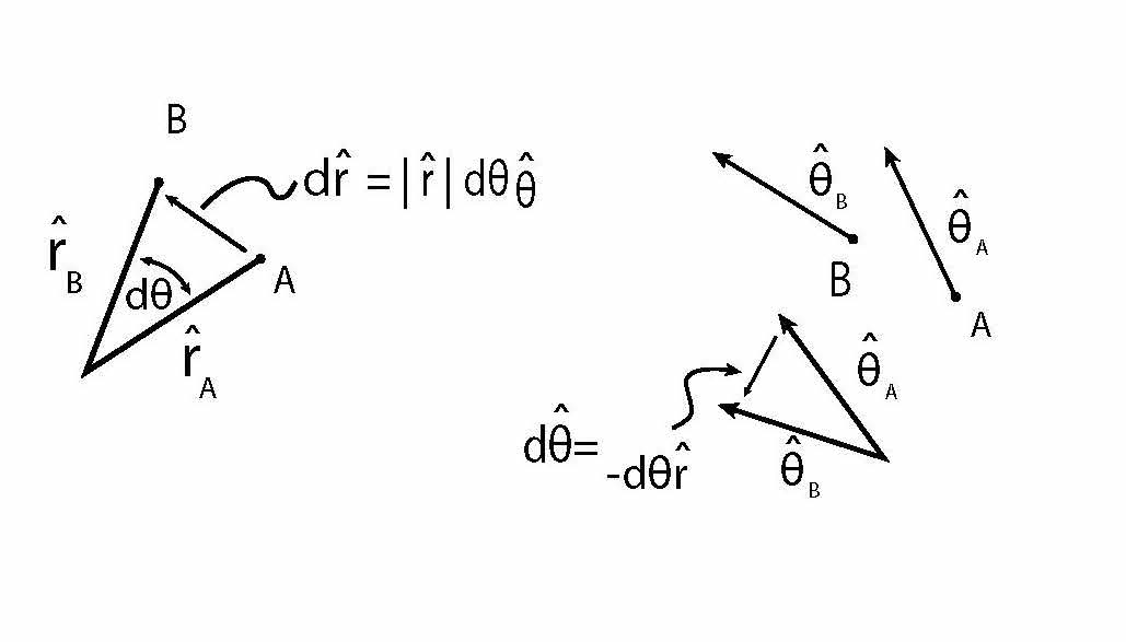
Similarly the change in the unit vector, \(d\hat{\theta}=-rd\theta\), as illustrated above on the right as well. This is negative because if the change in the unit vector is counterclockwise the change in the r unit vector is in the negative r direction. The result is \(\frac{\partial\hat{\theta}}{\partial\theta}=-r\).
All of this can now be combined and used in the material derivative above resulting in:
\[\frac{DV}{Dt}=\frac{\partial V}{\partial t}+u_r\frac{\partial V}{\partial r}+\frac{u_\theta\partial V}{r\partial\theta} = \left ( \frac{\partial u_r}{\partial t}+u_r\frac{\partial u_r}{\partial r}+\frac{\partial_\theta\partial u_r}{r\partial\theta}-\frac{u_\theta^2}{r} \right )\hat{r}+\left ( \frac{\partial u_\theta}{\partial t}+u_r\frac{\partial u_\theta}{\partial r}+\frac{u_\theta\partial u_\theta}{r \partial\theta}+\frac{u_r u_\theta}{r} \right )\hat{\theta}\]
This applies to Cylindrical Coordinates, but as we shall see helps to interpret streamline coordinates when there is curvature to the streamline. The net result is added terms that account for the change of the unit vectors due to the curving nature of the flow.
Acceleration
If one finds the material derivative of the velocity vector of a fixed mass of fluid, namely Eqn. 2.2, the result is the acceleration of that fixed mass of fluid in time and space. The general expression for this vector quantity can be written in tensor notation as:
\[\frac{Du_i}{Dt}=\frac{\partial u_i}{\partial t}+u_j\frac{\partial u_i}{\partial x_j}\label{2.4} \]
Note here that the vector, V is replaced with the tensor notation for a vector written as \({u{}_{i}}\). Also the summation rule has been used in the second term on the right hand side, this implies that there are really three terms being represented by the one term shown. The first term on the right hand side is denoted as the “local acceleration” and physically represents the rate change of velocity at a fixed point in space. The second expression on the right hand side is denoted as the “convective acceleration” and physically represents how the velocity field changes over space. If a flow is steady the local acceleration is by definition zero. However a fluid mass as it moves through space where the velocity changes in space will experience acceleration (or deceleration). An example is steady flow through a nozzle, or diffuser, where the fluid velocity will increase, or decrease, along the flow direction. For these two cases a fixed mass of fluid will accelerate, or decelerate due to moving in space. The reader is reminded that the components of the acceleration depend on the component of velocity in the derivatives.The convective acceleration can be rewritten using a vector identity listed above. Namely, the convective acceleration in vector notation is \(\left(V\cdot \mathrm{\nabla }\right)V\) and can be expressed as:\(\left(V\cdot \mathrm{\nabla }\right)V=\frac{1}{2}\mathrm{\nabla }\left(\mathrm{V}\mathrm{\cdot }\mathrm{V}\right)\mathrm{-}\mathrm{V\times (}\mathrm{\nabla }\mathrm{\times V)}\). In tensor notation this becomes:
\[u_j\frac{\partial u_i}{\partial x_j}=\frac{1}{2}\frac{\partial \left(u_ju_j\right)}{\partial x_j}-{\varepsilon }_{ijk}\left(u_j{\varepsilon }_{klm}\frac{\partial u_m}{\partial x_l}\right)\label{2.5} \]
Consequently, the convective acceleration can be recast as the expression on the right hand side. Although this may not seem like it is of any benefit and just makes things more complicated we will show that it does indeed have advantages. The reader should pay attention to the subscripts in the above expression. Notice that each term is a vector with the free index of “\({i}\)”, all other indices are repeated and therefore summed. In the summation of vectors we basically need to sum components, this implies that they have the same index, in this case “\({i}\)”.
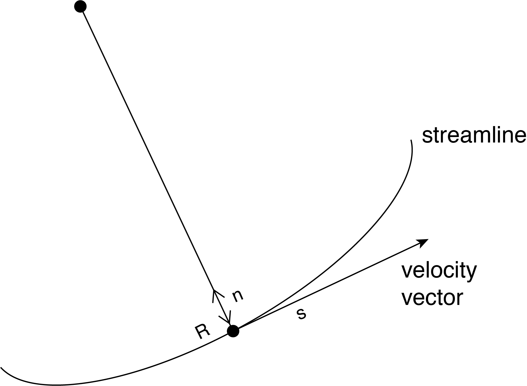
Streamline Coordinates
Streamline Coordinates define the flow direction of the velocity vector. It is defined as the locus of points tangent to the velocity vector at some instant in time. If the flow is steady these lines do not change. For our purposes we will consider steady flow here, but that is not necessary. Figure 2.1 illustrates the streamline as well as a streamline coordinate system we will define. Our discussion for simplicity will be two dimensional such that flow is within the \({s-n}\) plane. We retain an orthogonal coordinate system with “s” along the streamline and “n” normal to the streamline. The third coordinate would be normal to both \({s}\) and \({n}\), into the page.
If we take the cylindrical coordinate system as an example and consider flow along a curve, with some non-infinite radius of curvature, then we expect additional terms to appear in the acceleration. These terms account for the changing unit vectors as discussed in the material derivative in cylindrical coordinates. We make note of the fact that the velocity in the \({n}\) direction is zero, by definition of the streamline. However, there can still be acceleration in the \({n}\) direction since the unit vectors are changing. Using the cylindrical coordinate expression as a guide and denoting \({r}\) as normal to the streamline direction, \({n}\), and \({θ}\) as along the streamline direction, \({s}\), then the results for acceleration in the \({s}\) and \({n}\) directions are:
\[a_s=\frac{\partial u_s}{\partial t}+u_s\frac{\partial u_s}{\partial s}=\frac{\partial u_s}{\partial t}+\frac{\partial {u_s}^2}{2}\label{2.6} \]
\[a_n=\frac
Callstack:
    at (Bookshelves/Civil_Engineering/Intermediate_Fluid_Mechanics_(Liburdy)/02:_Mathematical_Tools), /content/body/div[3]/div[3]/p[4]/span, line 1, column 4
Here \({R}\) is the local value of the radius of curvature of the streamline. The value of \({R}\) goes to infinity for a straight streamline and there is no acceleration in the \({n}\) direction. Recall here that \({u{}_{r}}\) (or \({u{}_{n}}\)) is identically zero at the streamline and that the expression for \(a_n\)only contains the last term associated with the changing unit vector \({θ}\), or in this case \({s}\). Also we define in the streamline coordinates the direction \({n}\) to be inward towards the radius of curvature as shown in Figure 2.1. This is opposite to the convention used in cylindrical coordinates where \({r}\) is radially outward, hence the sign is positive for the value of \(a_n\). That is, if there is a curving streamline the acceleration is inward towards the direction of the center of the radius of curvature.
Velocity Gradient Tensor
The velocity gradient tensor describes how the velocity varies near a specified location within the flow field. It is represented as \(\frac{\partial u_j}{\partial x_i}\) which is a second order tensor, and therefor has nine components in three dimensional space. A second order tensor can be decomposed into symmetric and antisymmetric parts given as follows:
\[\frac{\partial u_j}{\partial x_i}=\frac{1}{2}\left(\frac{\partial u_j}{\partial x_i}\mathrm{\ }\mathrm{+}\frac{\partial u_i}{\partial x_j}\mathrm{\ }\right)+\frac{1}{2}\left(\frac{\partial u_j}{\partial x_i}\mathrm{\ }\mathrm{-}\frac{\partial u_i}{\partial x_j}\mathrm{\ }\right)\label{2.7} \]
Notice here that the first term adds half of the transpose of the original tensor and the second term subtracts the same quantity completing this identity. The first term is symmetric that is by inverting the \({i}\) and \({j}\) subscripts there is no change in the value of the element. The second term is antisymmetric such that inverting the subscripts the value of the element has the opposite sign. The ½ multiplier is included in the definition of the symmetric and antisymmetric parts such that their sum results in the original tensor.
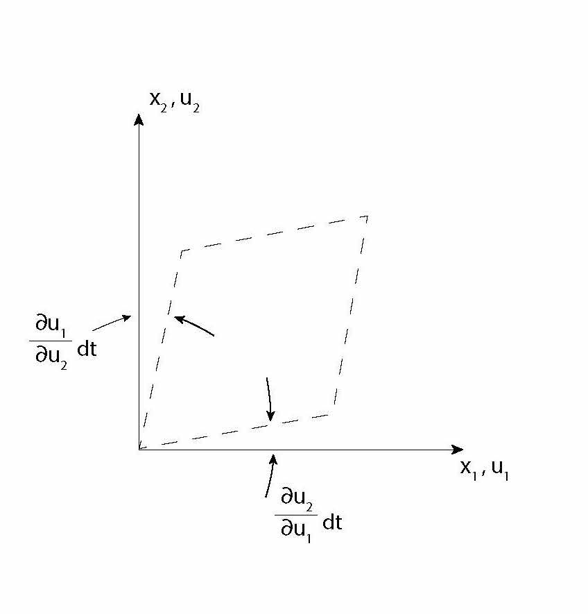
In fluid mechanics applications the velocity gradient tensor is a measure of the velocity changes experienced in the fluid flow as one moves away (infinitesimally) from a given point. That is to say this tensor is a point function, having a value at any given point in the flow. We refer to that as a local function in space. It may be time dependent as well. So we can say that this tensor has a symmetric part and an antisymmetric part. As we will see when we discuss the viscous forces within a fluid the symmetric part is representative of the deformation rate, or strain rate, experienced by a fluid element. The antisymmetric part represents the rotation rate of a fluid element. If one examines the curl operator on \({u{}_{j}}\) given previously as \({\varepsilon }_{kij}\frac{\partial u_j}{\partial x_i}\), where the subscripts indicate that this is the \({k}th\) element, it can be shown by writing out the terms of the curl operation on \({u{}_{j}}\) that this is equivalent to twice the antisymmetric part of \(\frac{\partial u_j}{\partial x_i}\) (or the part in parentheses of the second term in Equation \ref{2.7}). Therefore the rotation part of the velocity gradient tensor is one half the vorticity of the flow. To be clear, the antisymmetric part of \(\frac{\partial u_j}{\partial x_i}\) is a second order tensor, but from observation if i=j then the value of this is identically zero (all zero components along the diagonal of the tensor). The off diagonal terms are six in total but those with inverted indices are the negatives of the noninverted components (\(\frac{\partial u_j}{\partial x_i}=-\frac{\partial u_i}{\partial x_j}\)). Consequently there are only three independent values, so we identify this second order tensor as a pseudo-vector, having three components. It is a so called pseudo-vector since the sign is arbitrary. In other words do we set \(\frac{\partial u_1}{\partial x_2}\) as a positive or negative quantity? The sign convention is typically selected so that a counter clockwise rotation is a positive value. This means that for \(\frac{\partial u_1}{\partial x_2}\) being positive then as \({u{}_{1}}\) increases in the positive \({x{}_{2}}\) direction then the flow will tend to rotate clockwise and is a negative rotation direction. This is illustrated in Figure 2.2. Note that if one considers a negative value of \(\frac{\partial u_1}{\partial x_2}\) coupled with a positive value of \(\frac{\partial u_2}{\partial x_1}\) such that
\[{\omega_3}=\left (\frac {\partial u_2}{\partial x_1} -\frac {\partial u_1}{\partial x_2} \right)\label{2.8} \]
then rotation (or vorticity) about the 3 axis (out of the page in Figure 2.2) is counterclockwise. Obviously, the signs of the two components of the velocity gradient that go into any of the vorticity components can be positive and/or negative. If in the above example for Eqn. 2.8 the magnitudes of \(\frac{\partial u_2}{\partial x_1}\) and \(\frac{\partial u_1}{\partial x_2}\) are equal and their signs are the same then the vorticity component \({\omega }{_3}\) will be zero. One can think of the net vorticity or rotation rate vector component to be the combined value from both velocity derivative components, which contribute to rotation about an axis. The same interpretation of the combined effects of the two velocity gradient elements can be made for the strain rate, or the symmetric part of the velocity gradient tensor. When the rotation rates of the vertical and horizontal axes are identical (both elements causing, say, counterclockwise rotation at the same rate) then the strain rate will be zero (the two elements in the symmetric part cancel) and the flow is in pure rotation, as a solid body.
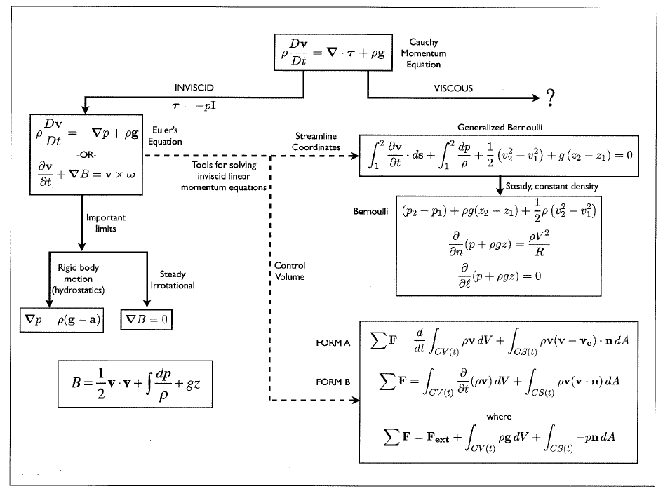
Basic Equations
The basic equations generally used in inviscid fluid mechanics are shown in Figure 2.3. The viscous terms we will add later. But this chart shows various forms of the governing momentum equation which include pressure and gravitational forces contributing to the overall acceleration of the fluid. At the top is the basic Cauchy form of the momentum equation, where viscous effects would be contained in the stress term, \(τ\). The inclusion of viscous terms will be developed in a later chapter. At this point the stress only contains the pressure forces, which is compressive and normal. The streamline coordinate formulation is shown on the right where integration is along the streamline. The introduction of the variable B is a consequence of using the last of the vector identities listed above as equation (2.5) for the convective acceleration term, and then combining the terms shown in the bottom box on the left. Here B is essentially the Bernoulli constant for steady, compressible flow. This is discussed further in the development of the Bernoulli equation. At this point the equations are presented for reference later on when the various terms are developed.