14.4: Solving Systems of Linear Equations

Last updated
Save as PDF

Page ID: 15002

\( \newcommand{\vecs}[1]{\overset { \scriptstyle \rightharpoonup} {\mathbf{#1}} } \) \( \newcommand{\vecd}[1]{\overset{-\!-\!\rightharpoonup}{\vphantom{a}\smash {#1}}} \)\(\newcommand{\id}{\mathrm{id}}\) \( \newcommand{\Span}{\mathrm{span}}\) \( \newcommand{\kernel}{\mathrm{null}\,}\) \( \newcommand{\range}{\mathrm{range}\,}\) \( \newcommand{\RealPart}{\mathrm{Re}}\) \( \newcommand{\ImaginaryPart}{\mathrm{Im}}\) \( \newcommand{\Argument}{\mathrm{Arg}}\) \( \newcommand{\norm}[1]{\| #1 \|}\) \( \newcommand{\inner}[2]{\langle #1, #2 \rangle}\) \( \newcommand{\Span}{\mathrm{span}}\) \(\newcommand{\id}{\mathrm{id}}\) \( \newcommand{\Span}{\mathrm{span}}\) \( \newcommand{\kernel}{\mathrm{null}\,}\) \( \newcommand{\range}{\mathrm{range}\,}\) \( \newcommand{\RealPart}{\mathrm{Re}}\) \( \newcommand{\ImaginaryPart}{\mathrm{Im}}\) \( \newcommand{\Argument}{\mathrm{Arg}}\) \( \newcommand{\norm}[1]{\| #1 \|}\) \( \newcommand{\inner}[2]{\langle #1, #2 \rangle}\) \( \newcommand{\Span}{\mathrm{span}}\)\(\newcommand{\AA}{\unicode[.8,0]{x212B}}\)

Suppose we have the following system of linear equations.

\[3w-x+y+z=3\\-x-y+3z=1\\5w+3x-y-z=-1\\2w+2x-y=0\nonumber\]

The goal is to solve them simultaneously for the variables w, x, y and z. Assuming that there is exactly one answer (i.e. one quadruple for w, x, y, z) then there are many ways to do this. Here we use rref, lsolve and the matrix inverse as examples.

rref

The command rref is short for “reduced row echelon form.” Through a process called Gaussian elimination the matrix of coefficients (on w, x, y, z) augmented by the matrix of constants (the numbers on the right of the equals signs) is reduced to a matrix of zeros and ones (the “identity matrix”) together with the solution (in the last column). In the matrix a, we store the cofficients for w in the first column, x in the second column, y in the third column, z in the fourth column and the constants in the fifth column. If a variable does not occur in an equation, a zero is in the corresponding entry of the matrix a.

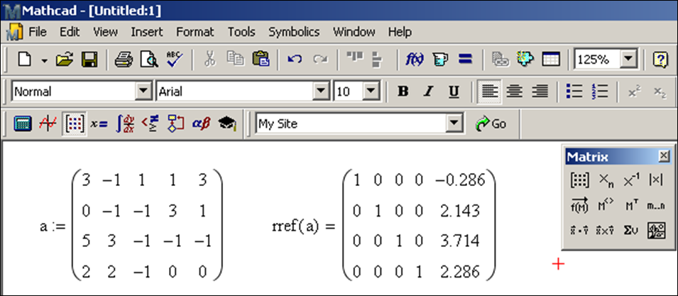
The last column indicates that the only solution to the system of equations is w = −0.286, x = 2.143, y = 3.714, z = 2.286 to three place decimal accuracy. Recall, for more decimal places, select Format > Result or simply double click the equation.

lsolve

To use the command lsolve, we need two separate matrices, one with the coefficients of w, x, y, z and one with the constants to the right side of the equals sign. We could input this from scratch or practice referencing them from the matrix a above. Here is the syntax for how to use the lsolve command.

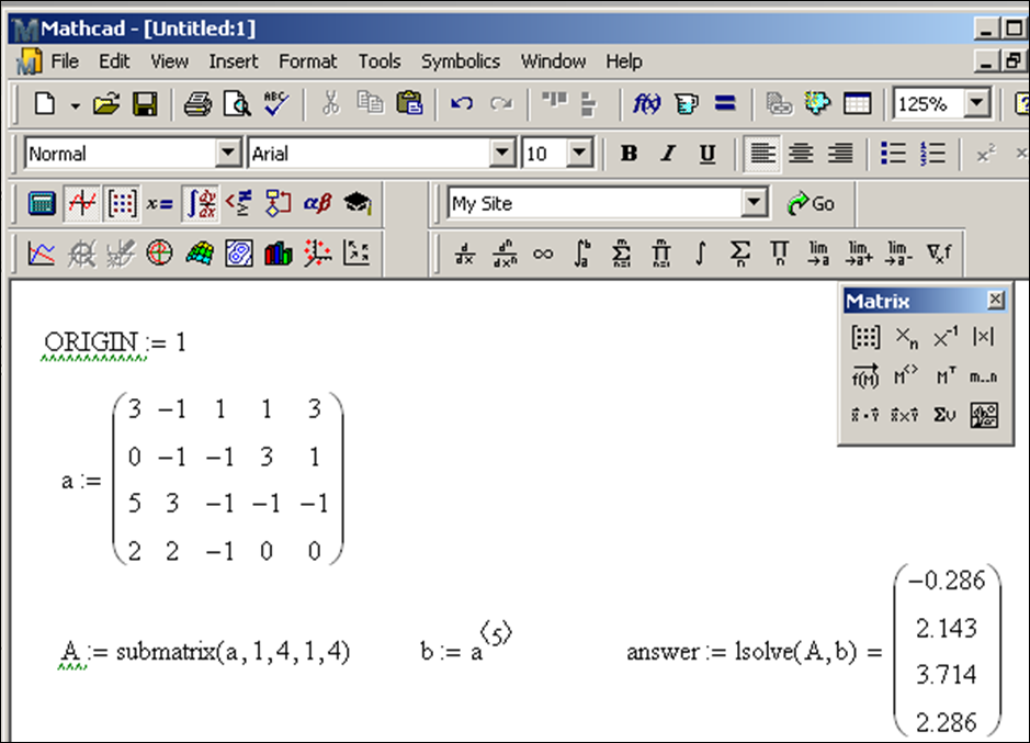
The variable answer contains the only solution to the system of equations as w = −0.286, x = 2.143, y = 3.714, z = 2.286.

Using the matrix inverse

The setup for the using the inverse of a matrix is similar as for using lsolve. We need the coefficient matrix of w, x, y, z and the constant matrix. The inverse
of a matrix is found by typing the name of the matrix and then selecting the x^-1 button. When entering the equation for the variable answer, make sure that b is multiplying correctly. Here is the sequence of commands:

answer : A x^-1(spacebar) (spacebar) b =

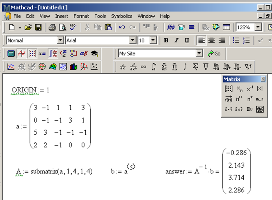
The variable answer contains the only solution to the system of equations as w = −0.286, x = 2.143, y = 3.714, z = 2.286. You might be wondering “if there are several methods to find the solution, then which technique should you use?” The answer is (of course) more complex than we will go into here, but leave it to say that some techniques are faster or more accurate than others. In fact if a system is either “non-square” (has a different number of equations and variables) or the coefficient matrix is “singular” (look it up) then the lsolve and inverse techniques don’t work and in this case the system of equations either has no solution (“inconsistent”) or has infinitely many solutions (“underdetermined”). Ok, enough theory.