1.5: A simple network to classify handwritten digits

Having defined neural networks, let's return to handwriting recognition. We can split the problem of recognizing handwritten digits into two sub-problems. First, we'd like a way of breaking an image containing many digits into a sequence of separate images, each containing a single digit. For example, we'd like to break the image

into six separate images,

We humans solve this segmentation problem with ease, but it's challenging for a computer program to correctly break up the image. Once the image has been segmented, the program then needs to classify each individual digit. So, for instance, we'd like our program to recognize that the first digit above,

is a 5.

We'll focus on writing a program to solve the second problem, that is, classifying individual digits. We do this because it turns out that the segmentation problem is not so difficult to solve, once you have a good way of classifying individual digits. There are many approaches to solving the segmentation problem. One approach is to trial many different ways of segmenting the image, using the individual digit classifier to score each trial segmentation. A trial segmentation gets a high score if the individual digit classifier is confident of its classification in all segments, and a low score if the classifier is having a lot of trouble in one or more segments. The idea is that if the classifier is having trouble somewhere, then it's probably having trouble because the segmentation has been chosen incorrectly. This idea and other variations can be used to solve the segmentation problem quite well. So instead of worrying about segmentation we'll concentrate on developing a neural network which can solve the more interesting and difficult problem, namely, recognizing individual handwritten digits.

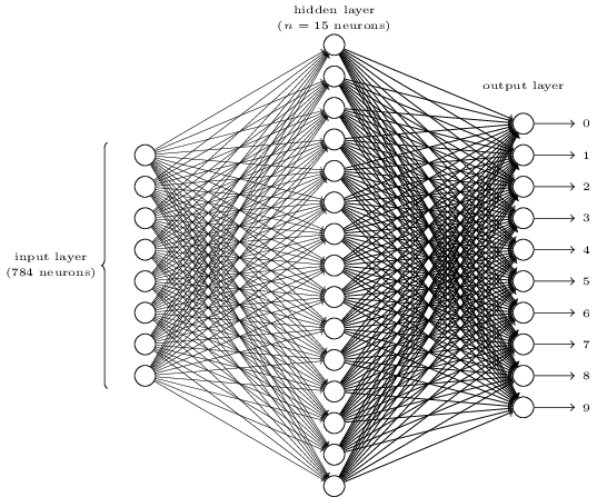
To recognize individual digits we will use a three-layer neural network:

The input layer of the network contains neurons encoding the values of the input pixels. As discussed in the next section, our training data for the network will consist of many \(28 by 28\) pixel images of scanned handwritten digits, and so the input layer contains \(784 = 28×28\) neurons. For simplicity I've omitted most of the \(784\) input neurons in the diagram above. The input pixels are greyscale, with a value of \(0.0\) representing white, a value of \(1.0\) representing black, and in between values representing gradually darkening shades of grey.

The second layer of the network is a hidden layer. We denote the number of neurons in this hidden layer by \(n\), and we'll experiment with different values for \(n\). The example shown illustrates a small hidden layer, containing just \(n=15\) neurons.

The output layer of the network contains \(10 neurons\). If the first neuron fires, i.e., has an \(output ≈1\), then that will indicate that the network thinks the digit is a \(0\). If the second neuron fires then that will indicate that the network thinks the digit is a \(1\). And so on. A little more precisely, we number the output neurons from \(0\) through \(9\), and figure out which neuron has the highest activation value. If that neuron is, say, neuron number \(6\), then our network will guess that the input digit was a \(6\). And so on for the other output neurons.

You might wonder why we use \(10\) output neurons. After all, the goal of the network is to tell us which digit \((0,1,2,…,9)\) corresponds to the input image. A seemingly natural way of doing that is to use just \(4\) output neurons, treating each neuron as taking on a binary value, depending on whether the neuron's output is closer to \(0\) or to \(1\). Four neurons are enough to encode the answer, since \(2^4 = 16\) is more than the \(10\) possible values for the input digit. Why should our network use \(10\) neurons instead? Isn't that inefficient? The ultimate justification is empirical: we can try out both network designs, and it turns out that, for this particular problem, the network with \(10\) output neurons learns to recognize digits better than the network with \(4\) output neurons. But that leaves us wondering why using \(10\) output neurons works better. Is there some heuristic that would tell us in advance that we should use the \(10-output\) encoding instead of the \(4-output\) encoding?

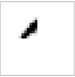
To understand why we do this, it helps to think about what the neural network is doing from first principles. Consider first the case where we use \(10\) output neurons. Let's concentrate on the first output neuron, the one that's trying to decide whether or not the digit is a \(0\). It does this by weighing up evidence from the hidden layer of neurons. What are those hidden neurons doing? Well, just suppose for the sake of argument that the first neuron in the hidden layer detects whether or not an image like the following is present:

It can do this by heavily weighting input pixels which overlap with the image, and only lightly weighting the other inputs. In a similar way, let's suppose for the sake of argument that the second, third, and fourth neurons in the hidden layer detect whether or not the following images are present:

As you may have guessed, these four images together make up the 0 image that we saw in the line of digits shown earlier:

So if all four of these hidden neurons are firing then we can conclude that the digit is a \(0\). Of course, that's not the only sort of evidence we can use to conclude that the image was a \(0\).we could legitimately get a \(0\) in many other ways (say, through translations of the above images, or slight distortions). But it seems safe to say that at least in this case we'd conclude that the input was a \(0\).

Supposing the neural network functions in this way, we can give a plausible explanation for why it's better to have \(10\) outputs from the network, rather than \(4\). If we had \(4\) outputs then the first output neuron would be trying to decide what the most significant bit of the digit was. And there's no easy way to relate that most significant bit to simple shapes like those shown above. It's hard to imagine that there's any good historical reason the component shapes of the digit will be closely related to (say) the most significant bit in the output.

Now, with all that said, this is all just a heuristic. Nothing says that the three-layer neural network has to operate in the way I described, with the hidden neurons detecting simple component shapes. Maybe a clever learning algorithm will find some assignment of weights that lets us use only \(4\) output neurons. But as a heuristic the way of thinking I've described works pretty well, and can save you a lot of time in designing good neural network architectures.

Exercise

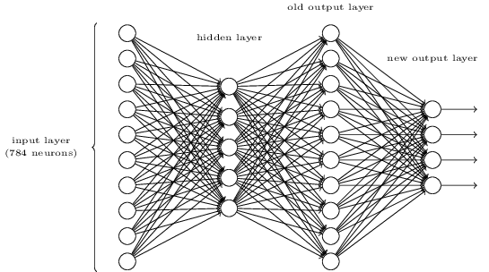
• There is a way of determining the bitwise representation of a digit by adding an extra layer to the three-layer network above. The extra layer converts the output from the previous layer into a binary representation, as illustrated in the figure below. Find a set of weights and biases for the new output layer. Assume that the first \(3\) layers of neurons are such that the correct output in the third layer (i.e., the old output layer) has activation at least \(0.99\),and incorrect outputs have activation less than \(0.01\).