10.1: BinaryHeap - An Implicit Binary Tree
- Page ID
- 8477
\( \newcommand{\vecs}[1]{\overset { \scriptstyle \rightharpoonup} {\mathbf{#1}} } \)
\( \newcommand{\vecd}[1]{\overset{-\!-\!\rightharpoonup}{\vphantom{a}\smash {#1}}} \)
\( \newcommand{\id}{\mathrm{id}}\) \( \newcommand{\Span}{\mathrm{span}}\)
( \newcommand{\kernel}{\mathrm{null}\,}\) \( \newcommand{\range}{\mathrm{range}\,}\)
\( \newcommand{\RealPart}{\mathrm{Re}}\) \( \newcommand{\ImaginaryPart}{\mathrm{Im}}\)
\( \newcommand{\Argument}{\mathrm{Arg}}\) \( \newcommand{\norm}[1]{\| #1 \|}\)
\( \newcommand{\inner}[2]{\langle #1, #2 \rangle}\)
\( \newcommand{\Span}{\mathrm{span}}\)
\( \newcommand{\id}{\mathrm{id}}\)
\( \newcommand{\Span}{\mathrm{span}}\)
\( \newcommand{\kernel}{\mathrm{null}\,}\)
\( \newcommand{\range}{\mathrm{range}\,}\)
\( \newcommand{\RealPart}{\mathrm{Re}}\)
\( \newcommand{\ImaginaryPart}{\mathrm{Im}}\)
\( \newcommand{\Argument}{\mathrm{Arg}}\)
\( \newcommand{\norm}[1]{\| #1 \|}\)
\( \newcommand{\inner}[2]{\langle #1, #2 \rangle}\)
\( \newcommand{\Span}{\mathrm{span}}\) \( \newcommand{\AA}{\unicode[.8,0]{x212B}}\)
\( \newcommand{\vectorA}[1]{\vec{#1}} % arrow\)
\( \newcommand{\vectorAt}[1]{\vec{\text{#1}}} % arrow\)
\( \newcommand{\vectorB}[1]{\overset { \scriptstyle \rightharpoonup} {\mathbf{#1}} } \)
\( \newcommand{\vectorC}[1]{\textbf{#1}} \)
\( \newcommand{\vectorD}[1]{\overrightarrow{#1}} \)
\( \newcommand{\vectorDt}[1]{\overrightarrow{\text{#1}}} \)
\( \newcommand{\vectE}[1]{\overset{-\!-\!\rightharpoonup}{\vphantom{a}\smash{\mathbf {#1}}}} \)
\( \newcommand{\vecs}[1]{\overset { \scriptstyle \rightharpoonup} {\mathbf{#1}} } \)
\( \newcommand{\vecd}[1]{\overset{-\!-\!\rightharpoonup}{\vphantom{a}\smash {#1}}} \)
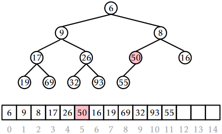
\(\newcommand{\avec}{\mathbf a}\) \(\newcommand{\bvec}{\mathbf b}\) \(\newcommand{\cvec}{\mathbf c}\) \(\newcommand{\dvec}{\mathbf d}\) \(\newcommand{\dtil}{\widetilde{\mathbf d}}\) \(\newcommand{\evec}{\mathbf e}\) \(\newcommand{\fvec}{\mathbf f}\) \(\newcommand{\nvec}{\mathbf n}\) \(\newcommand{\pvec}{\mathbf p}\) \(\newcommand{\qvec}{\mathbf q}\) \(\newcommand{\svec}{\mathbf s}\) \(\newcommand{\tvec}{\mathbf t}\) \(\newcommand{\uvec}{\mathbf u}\) \(\newcommand{\vvec}{\mathbf v}\) \(\newcommand{\wvec}{\mathbf w}\) \(\newcommand{\xvec}{\mathbf x}\) \(\newcommand{\yvec}{\mathbf y}\) \(\newcommand{\zvec}{\mathbf z}\) \(\newcommand{\rvec}{\mathbf r}\) \(\newcommand{\mvec}{\mathbf m}\) \(\newcommand{\zerovec}{\mathbf 0}\) \(\newcommand{\onevec}{\mathbf 1}\) \(\newcommand{\real}{\mathbb R}\) \(\newcommand{\twovec}[2]{\left[\begin{array}{r}#1 \\ #2 \end{array}\right]}\) \(\newcommand{\ctwovec}[2]{\left[\begin{array}{c}#1 \\ #2 \end{array}\right]}\) \(\newcommand{\threevec}[3]{\left[\begin{array}{r}#1 \\ #2 \\ #3 \end{array}\right]}\) \(\newcommand{\cthreevec}[3]{\left[\begin{array}{c}#1 \\ #2 \\ #3 \end{array}\right]}\) \(\newcommand{\fourvec}[4]{\left[\begin{array}{r}#1 \\ #2 \\ #3 \\ #4 \end{array}\right]}\) \(\newcommand{\cfourvec}[4]{\left[\begin{array}{c}#1 \\ #2 \\ #3 \\ #4 \end{array}\right]}\) \(\newcommand{\fivevec}[5]{\left[\begin{array}{r}#1 \\ #2 \\ #3 \\ #4 \\ #5 \\ \end{array}\right]}\) \(\newcommand{\cfivevec}[5]{\left[\begin{array}{c}#1 \\ #2 \\ #3 \\ #4 \\ #5 \\ \end{array}\right]}\) \(\newcommand{\mattwo}[4]{\left[\begin{array}{rr}#1 \amp #2 \\ #3 \amp #4 \\ \end{array}\right]}\) \(\newcommand{\laspan}[1]{\text{Span}\{#1\}}\) \(\newcommand{\bcal}{\cal B}\) \(\newcommand{\ccal}{\cal C}\) \(\newcommand{\scal}{\cal S}\) \(\newcommand{\wcal}{\cal W}\) \(\newcommand{\ecal}{\cal E}\) \(\newcommand{\coords}[2]{\left\{#1\right\}_{#2}}\) \(\newcommand{\gray}[1]{\color{gray}{#1}}\) \(\newcommand{\lgray}[1]{\color{lightgray}{#1}}\) \(\newcommand{\rank}{\operatorname{rank}}\) \(\newcommand{\row}{\text{Row}}\) \(\newcommand{\col}{\text{Col}}\) \(\renewcommand{\row}{\text{Row}}\) \(\newcommand{\nul}{\text{Nul}}\) \(\newcommand{\var}{\text{Var}}\) \(\newcommand{\corr}{\text{corr}}\) \(\newcommand{\len}[1]{\left|#1\right|}\) \(\newcommand{\bbar}{\overline{\bvec}}\) \(\newcommand{\bhat}{\widehat{\bvec}}\) \(\newcommand{\bperp}{\bvec^\perp}\) \(\newcommand{\xhat}{\widehat{\xvec}}\) \(\newcommand{\vhat}{\widehat{\vvec}}\) \(\newcommand{\uhat}{\widehat{\uvec}}\) \(\newcommand{\what}{\widehat{\wvec}}\) \(\newcommand{\Sighat}{\widehat{\Sigma}}\) \(\newcommand{\lt}{<}\) \(\newcommand{\gt}{>}\) \(\newcommand{\amp}{&}\) \(\definecolor{fillinmathshade}{gray}{0.9}\)Our first implementation of a (priority) Queue is based on a technique that is over four hundred years old. Eytzinger's method allows us to represent a complete binary tree as an array by laying out the nodes of the tree in breadth-first order (see Section 6.1.2). In this way, the root is stored at position 0, the root's left child is stored at position 1, the root's right child at position 2, the left child of the left child of the root is stored at position 3, and so on. See Figure \(\PageIndex{1}\).
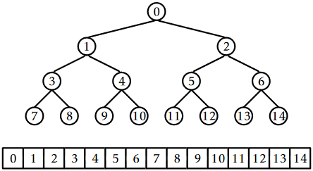
If we apply Eytzinger's method to a sufficiently large tree, some patterns emerge. The left child of the node at index \(\mathtt{i}\) is at index \(\mathtt{left(i)}=2\mathtt{i}+1\) and the right child of the node at index \(\mathtt{i}\) is at index \(\mathtt{right(i)}=2\mathtt{i}+2\). The parent of the node at index \(\mathtt{i}\) is at index \(\mathtt{parent(i)}=(\mathtt{i}-1)/2\).
    int left(int i) {
        return 2*i + 1;
    }
    int right(int i) {
        return 2*i + 2;
    }
    int parent(int i) {
        return (i-1)/2;
    }
A BinaryHeap uses this technique to implicitly represent a complete binary tree in which the elements are heap-ordered: The value stored at any index \(\mathtt{i}\) is not smaller than the value stored at index \(\mathtt{parent(i)}\), with the exception of the root value, \(\mathtt{i}=0\). It follows that the smallest value in the priority Queue is therefore stored at position 0 (the root).
In a BinaryHeap, the \(\mathtt{n}\) elements are stored in an array \(\mathtt{a}\):
    T[] a;
    int n;
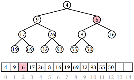
Implementing the \(\mathtt{add(x)}\) operation is fairly straightforward. As with all array-based structures, we first check to see if \(\mathtt{a}\) is full (by checking if \(\texttt{a.length}=\mathtt{n}\)) and, if so, we grow \(\mathtt{a}\). Next, we place \(\mathtt{x}\) at location \(\mathtt{a[n]}\) and increment \(\mathtt{n}\). At this point, all that remains is to ensure that we maintain the heap property. We do this by repeatedly swapping \(\mathtt{x}\) with its parent until \(\mathtt{x}\) is no longer smaller than its parent. See Figure \(\PageIndex{2}\).
    boolean add(T x) {
        if (n + 1 > a.length) resize();
        a[n++] = x;
        bubbleUp(n-1);
        return true;
    }
    void bubbleUp(int i) {
        int p = parent(i);
        while (i > 0 && compare(a[i], a[p]) < 0) {
            swap(i,p);
            i = p;
            p = parent(i);
        }
    }
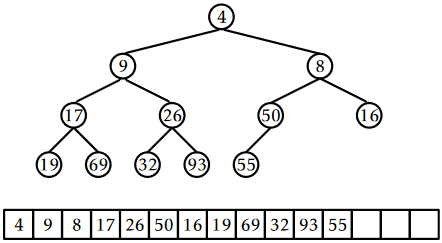
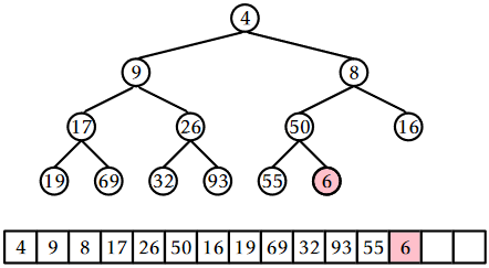
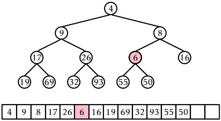
Implementing the \(\mathtt{remove()}\) operation, which removes the smallest value from the heap, is a little trickier. We know where the smallest value is (at the root), but we need to replace it after we remove it and ensure that we maintain the heap property.
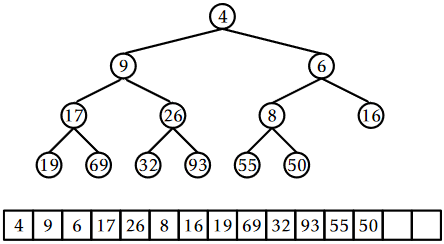
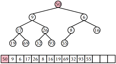
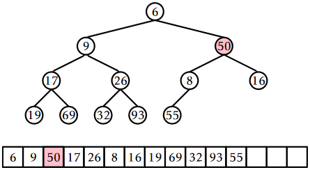
The easiest way to do this is to replace the root with the value \(\mathtt{a[n-1]}\), delete that value, and decrement \(\mathtt{n}\). Unfortunately, the new root element is now probably not the smallest element, so it needs to be moved downwards. We do this by repeatedly comparing this element to its two children. If it is the smallest of the three then we are done. Otherwise, we swap this element with the smallest of its two children and continue.
    T remove() {
        T x = a[0];
        a[0] = a[--n];
        trickleDown(0);
        if (3*n < a.length) resize();
        return x;
    }
    void trickleDown(int i) {
        do {
            int j = -1;
            int r = right(i);
            if (r < n && compare(a[r], a[i]) < 0) {
                int l = left(i);
                if (compare(a[l], a[r]) < 0) {
                    j = l;
                } else {
                    j = r;
                }
            } else {
                int l = left(i);
                if (l < n && compare(a[l], a[i]) < 0) {
                    j = l;
                }
            }
            if (j >= 0)    swap(i, j);
            i = j;
        } while (i >= 0);
    }
As with other array-based structures, we will ignore the time spent in calls to \(\mathtt{resize()}\), since these can be accounted for using the amortization argument from Lemma 2.1.1. The running times of both \(\mathtt{add(x)}\) and \(\mathtt{remove()}\) then depend on the height of the (implicit) binary tree. Luckily, this is a complete binary tree; every level except the last has the maximum possible number of nodes. Therefore, if the height of this tree is \(h\), then it has at least \(2^h\) nodes. Stated another way
\[ \mathtt{n} \ge 2^h \enspace . \nonumber\]
Taking logarithms on both sides of this equation gives
\[ h \le \log \mathtt{n} \enspace . \nonumber\]
Therefore, both the \(\mathtt{add(x)}\) and \(\mathtt{remove()}\) operation run in \(O(\log \mathtt{n})\) time.
\(\PageIndex{1}\) Summary
The following theorem summarizes the performance of a BinaryHeap:
A BinaryHeap implements the (priority) Queue interface. Ignoring the cost of calls to \(\mathtt{resize()}\), a BinaryHeap supports the operations \(\mathtt{add(x)}\) and \(\mathtt{remove()}\) in \(O(\log \mathtt{n})\) time per operation.
Furthermore, beginning with an empty BinaryHeap, any sequence of \(m\) \(\mathtt{add(x)}\) and \(\mathtt{remove()}\) operations results in a total of \(O(m)\) time spent during all calls to \(\mathtt{resize()}\).


