14.2: B-Trees

Last updated
Save as PDF

Page ID: 8496

$ \newcommand{\vecs}[1]{\overset { \scriptstyle \rightharpoonup} {\mathbf{#1}} } $ $ \newcommand{\vecd}[1]{\overset{-\!-\!\rightharpoonup}{\vphantom{a}\smash {#1}}} $$\newcommand{\id}{\mathrm{id}}$ $ \newcommand{\Span}{\mathrm{span}}$ $ \newcommand{\kernel}{\mathrm{null}\,}$ $ \newcommand{\range}{\mathrm{range}\,}$ $ \newcommand{\RealPart}{\mathrm{Re}}$ $ \newcommand{\ImaginaryPart}{\mathrm{Im}}$ $ \newcommand{\Argument}{\mathrm{Arg}}$ $ \newcommand{\norm}[1]{\| #1 \|}$ $ \newcommand{\inner}[2]{\langle #1, #2 \rangle}$ $ \newcommand{\Span}{\mathrm{span}}$ $\newcommand{\id}{\mathrm{id}}$ $ \newcommand{\Span}{\mathrm{span}}$ $ \newcommand{\kernel}{\mathrm{null}\,}$ $ \newcommand{\range}{\mathrm{range}\,}$ $ \newcommand{\RealPart}{\mathrm{Re}}$ $ \newcommand{\ImaginaryPart}{\mathrm{Im}}$ $ \newcommand{\Argument}{\mathrm{Arg}}$ $ \newcommand{\norm}[1]{\| #1 \|}$ $ \newcommand{\inner}[2]{\langle #1, #2 \rangle}$ $ \newcommand{\Span}{\mathrm{span}}$$\newcommand{\AA}{\unicode[.8,0]{x212B}}$

In this section, we discuss a generalization of binary trees, called $B$-trees, which is efficient in the external memory model. Alternatively, $B$-trees can be viewed as the natural generalization of 2-4 trees described in Section 9.1. (A 2-4 tree is a special case of a $B$-tree that we get by setting $B=2$.)

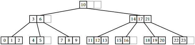
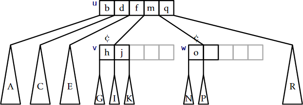
For any integer $B\ge 2$, a $B$-tree is a tree in which all of the leaves have the same depth and every non-root internal node, $\mathtt{u}$, has at least $B$ children and at most $2B$ children. The children of $\mathtt{u}$ are stored in an array, $\texttt{u.children}$. The required number of children is relaxed at the root, which can have anywhere between 2 and $2B$ children.

If the height of a $B$-tree is $h$, then it follows that the number, $\ell$, of leaves in the $B$-tree satisfies

\[ 2B^{h-1} \le \ell \le 2(2B)^{h-1} \enspace . \nonumber\]

Taking the logarithm of the first inequality and rearranging terms yields:

\[\begin{align}
h
&\le \frac{\log \ell-1}{\log B} + 1\nonumber\\
&\le \frac{\log \ell}{\log B} + 1\nonumber\\
&= \log_B \ell + 1 \enspace .\nonumber
\end{align}\nonumber\]

That is, the height of a $B$-tree is proportional to the base-$B$ logarithm of the number of leaves.

Each node, $\mathtt{u}$, in $B$-tree stores an array of keys $\texttt{u.keys}[0],\ldots,\texttt{u.keys}[2B-1]$. If $\mathtt{u}$ is an internal node with $k$ children, then the number of keys stored at $\mathtt{u}$ is exactly $k-1$ and these are stored in $\texttt{u.keys}[0],\ldots,\texttt{u.keys}[k-2]$. The remaining $2B-k+1$ array entries in $\texttt{u.keys}$ are set to $\mathtt{null}$. If $\mathtt{u}$ is a non-root leaf node, then $\mathtt{u}$ contains between $B-1$ and $2B-1$ keys. The keys in a $B$-tree respect an order similar to the keys in a binary search tree. For any node, $\mathtt{u}$, that stores $k-1$ keys,

\[ \texttt{u.keys[0]} < \texttt{u.keys[1]} < \cdots < \texttt{u.keys}[k-2] \enspace . \nonumber\]

If $\mathtt{u}$ is an internal node, then for every $\mathtt{i}\in\{0,\ldots,k-2\}$, $\texttt{u.keys[i]}$ is larger than every key stored in the subtree rooted at $\texttt{u.children[i]}$ but smaller than every key stored in the subtree rooted at $\mathtt{u.children[i+1]}$. Informally,

\[ \texttt{u.children[i]} \prec \texttt{u.keys[i]} \prec \mathtt{u.children[i+1]} \enspace . \nonumber\]

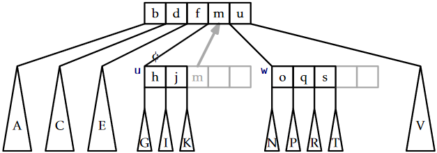
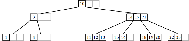
An example of a $B$-tree with $B=2$ is shown in Figure $\PageIndex{1}$.

Figure $\PageIndex{1}$: A $B$-tree with $B=2$.

Note that the data stored in a $B$-tree node has size $O(B)$. Therefore, in an external memory setting, the value of $B$ in a $B$-tree is chosen so that a node fits into a single external memory block. In this way, the time it takes to perform a $B$-tree operation in the external memory model is proportional to the number of nodes that are accessed (read or written) by the operation.

For example, if the keys are 4 byte integers and the node indices are also 4 bytes, then setting $B=256$ means that each node stores

\[ (4+4)\times 2B = 8\times512=4096 \nonumber\]

bytes of data. This would be a perfect value of $B$ for the hard disk or solid state drive discussed in the introduction to this chaper, which have a block size of $4096$ bytes.

The BTree class, which implements a $B$-tree, stores a BlockStore, $\mathtt{bs}$, that stores BTree nodes as well as the index, $\mathtt{ri}$, of the root node. As usual, an integer, $\mathtt{n}$, is used to keep track of the number of items in the data structure:

    int n;
    BlockStore<Node> bs;
    int ri;

$\PageIndex{1}$ Searching

The implementation of the $\mathtt{find(x)}$ operation, which is illustrated in Figure $\PageIndex{2}$, generalizes the $\mathtt{find(x)}$ operation in a binary search tree. The search for $\mathtt{x}$ starts at the root and uses the keys stored at a node, $\mathtt{u}$, to determine in which of $\mathtt{u}$'s children the search should continue.

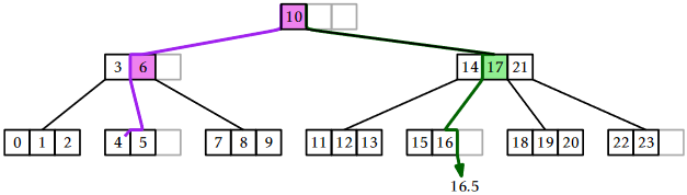
Figure $\PageIndex{2}$: A successful search (for the value 4) and an unsuccessful search (for the value 16.5) in a $B$-tree. Shaded nodes show where the value of $\mathtt{z}$ is updated during the searches.

More specifically, at a node $\mathtt{u}$, the search checks if $\mathtt{x}$ is stored in $\texttt{u.keys}$. If so, $\mathtt{x}$ has been found and the search is complete. Otherwise, the search finds the smallest integer, $\mathtt{i}$, such that $\texttt{u.keys[i]} > \mathtt{x}$ and continues the search in the subtree rooted at $\texttt{u.children[i]}$. If no key in $\texttt{u.keys}$ is greater than $\mathtt{x}$, then the search continues in $\mathtt{u}$'s rightmost child. Just like binary search trees, the algorithm keeps track of the most recently seen key, $\mathtt{z}$, that is larger than $\mathtt{x}$. In case $\mathtt{x}$ is not found, $\mathtt{z}$ is returned as the smallest value that is greater or equal to $\mathtt{x}$.

    T find(T x) {
        T z = null;
        int ui = ri;
        while (ui >= 0) {
            Node u = bs.readBlock(ui);
            int i = findIt(u.keys, x);
            if (i < 0) return u.keys[-(i+1)]; // found it
            if (u.keys[i] != null)
                z = u.keys[i];
            ui = u.children[i];
        }
        return z;
    }

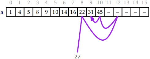
Central to the $\mathtt{find(x)}$ method is the $\mathtt{findIt(a,x)}$ method that searches in a $\mathtt{null}$-padded sorted array, $\mathtt{a}$, for the value $\mathtt{x}$. This method, illustrated in Figure $\PageIndex{3}$, works for any array, $\mathtt{a}$, where $\mathtt{a}[0],\ldots,\mathtt{a}[k-1]$ is a sequence of keys in sorted order and $\mathtt{a}[k],\ldots,\mathtt{a}[\texttt{a.length}-1]$ are all set to $\mathtt{null}$. If $\mathtt{x}$ is in the array at position $\mathtt{i}$, then $\mathtt{findIt(a,x)}$ returns $-\mathtt{i}-1$. Otherwise, it returns the smallest index, $\mathtt{i}$, such that $\mathtt{a[i]}>\mathtt{x}$ or $\mathtt{a[i]}=\mathtt{null}$.

Figure $\PageIndex{3}$: The execution of $\mathtt{findIt(a,27)}$.

    int findIt(T[] a, T x) {
        int lo = 0, hi = a.length;
        while (hi != lo) {
            int m = (hi+lo)/2;
            int cmp = a[m] == null ? -1 : compare(x, a[m]);
            if (cmp < 0)
                hi = m;      // look in first half
            else if (cmp > 0)
                lo = m+1;    // look in second half
            else
                return -m-1; // found it
        }
        return lo;
    }

The $\mathtt{findIt(a,x)}$ method uses a binary search that halves the search space at each step, so it runs in $O(\log(\texttt{a.length}))$ time. In our setting, $\texttt{a.length}=2B$, so $\mathtt{findIt(a,x)}$ runs in $O(\log B)$ time.

We can analyze the running time of a $B$-tree $\mathtt{find(x)}$ operation both in the usual word-RAM model (where every instruction counts) and in the external memory model (where we only count the number of nodes accessed). Since each leaf in a $B$-tree stores at least one key and the height of a $B$-Tree with $\ell$ leaves is $O(\log_B\ell)$, the height of a $B$-tree that stores $\mathtt{n}$ keys is $O(\log_B \mathtt{n})$. Therefore, in the external memory model, the time taken by the $\mathtt{find(x)}$ operation is $O(\log_B \mathtt{n})$. To determine the running time in the word-RAM model, we have to account for the cost of calling $\mathtt{findIt(a,x)}$ for each node we access, so the running time of $\mathtt{find(x)}$ in the word-RAM model is

\[ O(\log_B \mathtt{n})\times O(\log B) = O(\log \mathtt{n}) \enspace . \nonumber\]

$\PageIndex{2}$ Addition

One important difference between $B$-trees and the BinarySearchTree data structure from Section 6.2 is that the nodes of a $B$-tree do not store pointers to their parents. The reason for this will be explained shortly. The lack of parent pointers means that the $\mathtt{add(x)}$ and $\mathtt{remove(x)}$ operations on $B$-trees are most easily implemented using recursion.

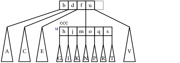
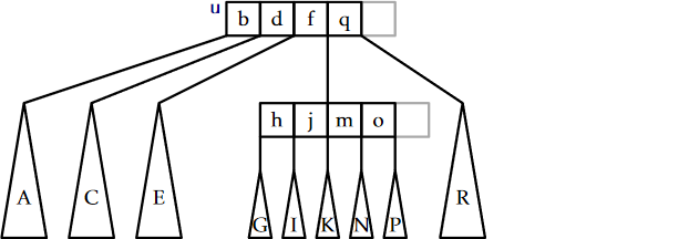
Like all balanced search trees, some form of rebalancing is required during an $\mathtt{add(x)}$ operation. In a $B$-tree, this is done by splitting nodes. Refer to Figure $\PageIndex{4}$ for what follows. Although splitting takes place across two levels of recursion, it is best understood as an operation that takes a node $\mathtt{u}$ containing $2B$ keys and having $2B+1$ children. It creates a new node, $\mathtt{w}$, that adopts $\texttt{u.children}[B],\ldots,\texttt{u.children}[2B]$. The new node $\mathtt{w}$ also takes $\mathtt{u}$'s $B$ largest keys, $\texttt{u.keys}[B],\ldots,\texttt{u.keys}[2B-1]$. At this point, $\mathtt{u}$ has $B$ children and $B$ keys. The extra key, $\texttt{u.keys}[B-1]$, is passed up to the parent of $\mathtt{u}$, which also adopts $\mathtt{w}$.

Notice that the splitting operation modifies three nodes: $\mathtt{u}$, $\mathtt{u}$'s parent, and the new node, $\mathtt{w}$. This is why it is important that the nodes of a $B$-tree do not maintain parent pointers. If they did, then the $B+1$ children adopted by $\mathtt{w}$ would all need to have their parent pointers modified. This would increase the number of external memory accesses from 3 to $B+4$ and would make $B$-trees much less efficient for large values of $B$.

Figure $\PageIndex{4}$: Splitting the node $\mathtt{u}$ in a $B$-tree ($B=3$). Notice that the key $\texttt{u.keys}[2]=\mathrm{m}$ passes from $\mathtt{u}$ to its parent.

The $\mathtt{add(x)}$ method in a $B$-tree is illustrated in Figure $\PageIndex{5}$. At a high level, this method finds a leaf, $\mathtt{u}$, at which to add the value $\mathtt{x}$. If this causes $\mathtt{u}$ to become overfull (because it already contained $B-1$ keys), then $\mathtt{u}$ is split. If this causes $\mathtt{u}$'s parent to become overfull, then $\mathtt{u}$'s parent is also split, which may cause $\mathtt{u}$'s grandparent to become overfull, and so on. This process continues, moving up the tree one level at a time until reaching a node that is not overfull or until the root is split. In the former case, the process stops. In the latter case, a new root is created whose two children become the nodes obtained when the original root was split.

Figure $\PageIndex{5}$: The $\mathtt{add(x)}$ operation in a `BTree`. Adding the value 21 results in two nodes being split.

The executive summary of the $\mathtt{add(x)}$ method is that it walks from the root to a leaf searching for $\mathtt{x}$, adds $\mathtt{x}$ to this leaf, and then walks back up to the root, splitting any overfull nodes it encounters along the way. With this high level view in mind, we can now delve into the details of how this method can be implemented recursively.

The real work of $\mathtt{add(x)}$ is done by the $\mathtt{addRecursive(x,ui)}$ method, which adds the value $\mathtt{x}$ to the subtree whose root, $\mathtt{u}$, has the identifier $\mathtt{ui}$. If $\mathtt{u}$ is a leaf, then $\mathtt{x}$ is simply inserted into $\texttt{u.keys}$. Otherwise, $\mathtt{x}$ is added recursively into the appropriate child, $\mathtt{u}'$, of $\mathtt{u}$. The result of this recursive call is normally $\mathtt{null}$ but may also be a reference to a newly-created node, $\mathtt{w}$, that was created because $\mathtt{u}'$ was split. In this case, $\mathtt{u}$ adopts $\mathtt{w}$ and takes its first key, completing the splitting operation on $\mathtt{u}'$.

After the value $\mathtt{x}$ has been added (either to $\mathtt{u}$ or to a descendant of $\mathtt{u}$), the $\mathtt{addRecursive(x,ui)}$ method checks to see if $\mathtt{u}$ is storing too many (more than $2B-1$) keys. If so, then $\mathtt{u}$ needs to be split with a call to the $\texttt{u.split()}$ method. The result of calling $\texttt{u.split()}$ is a new node that is used as the return value for $\mathtt{addRecursive(x,ui)}$.

    Node addRecursive(T x, int ui) throws DuplicateValueException {
        Node u = bs.readBlock(ui);
        int i = findIt(u.keys, x);
        if (i < 0) throw new DuplicateValueException();
        if (u.children[i] < 0) { // leaf node, just add it
            u.add(x, -1);
            bs.writeBlock(u.id, u);
        } else {
            Node w = addRecursive(x, u.children[i]);
            if (w != null) {  // child was split, w is new child 
                x = w.remove(0);
                bs.writeBlock(w.id, w);
                u.add(x, w.id);
                bs.writeBlock(u.id, u);
            }
        }
        return u.isFull() ? u.split() : null;
    }

The $\mathtt{addRecursive(x,ui)}$ method is a helper for the $\mathtt{add(x)}$ method, which calls $\mathtt{addRecursive(x,ri)}$ to insert $\mathtt{x}$ into the root of the $B$-tree. If $\mathtt{addRecursive(x,ri)}$ causes the root to split, then a new root is created that takes as its children both the old root and the new node created by the splitting of the old root.

    boolean add(T x) {
        Node w;
        try {
            w = addRecursive(x, ri);
        } catch (DuplicateValueException e) {
            return false;
        }
        if (w != null) {   // root was split, make new root
            Node newroot = new Node();
            x = w.remove(0);
            bs.writeBlock(w.id, w);
            newroot.children[0] = ri;
            newroot.keys[0] = x;
            newroot.children[1] = w.id;
            ri = newroot.id;
            bs.writeBlock(ri, newroot);
        }
        n++;
        return true;
    }

The $\mathtt{add(x)}$ method and its helper, $\mathtt{addRecursive(x,ui)}$, can be analyzed in two phases:

Downward phase:

During the downward phase of the recursion, before $\mathtt{x}$ has been added, they access a sequence of BTree nodes and call $\mathtt{findIt(a,x)}$ on each node. As with the $\mathtt{find(x)}$ method, this takes $O(\log_B \mathtt{n})$ time in the external memory model and $O(\log \mathtt{n})$ time in the word-RAM model.

Upward phase:

During the upward phase of the recursion, after $\mathtt{x}$ has been added, these methods perform a sequence of at most $O(\log_B \mathtt{n})$ splits. Each split involves only three nodes, so this phase takes $O(\log_B \mathtt{n})$ time in the external memory model. However, each split involves moving $B$ keys and children from one node to another, so in the word-RAM model, this takes $O(B\log \mathtt{n})$ time.

Recall that the value of $B$ can be quite large, much larger than even $\log \mathtt{n}$. Therefore, in the word-RAM model, adding a value to a $B$-tree can be much slower than adding into a balanced binary search tree. Later, in Section 14.2.4, we will show that the situation is not quite so bad; the amortized number of split operations done during an $\mathtt{add(x)}$ operation is constant. This shows that the (amortized) running time of the $\mathtt{add(x)}$ operation in the word-RAM model is $O(B+\log \mathtt{n})$.

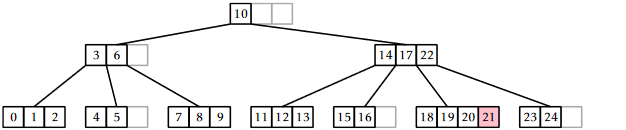
$\PageIndex{3}$ Removal

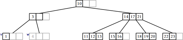
The $\mathtt{remove(x)}$ operation in a BTree is, again, most easily implemented as a recursive method. Although the recursive implementation of $\mathtt{remove(x)}$ spreads the complexity across several methods, the overall process, which is illustrated in Figure $\PageIndex{6}$, is fairly straightforward. By shuffling keys around, removal is reduced to the problem of removing a value, $\mathtt{x}'$, from some leaf, $\mathtt{u}$. Removing $\mathtt{x}'$ may leave $\mathtt{u}$ with less than $B-1$ keys; this situation is called an underflow.

Figure $\PageIndex{6}$: Removing the value 4 from a $B$-tree results in one merge and one borrowing operation.

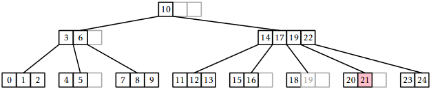
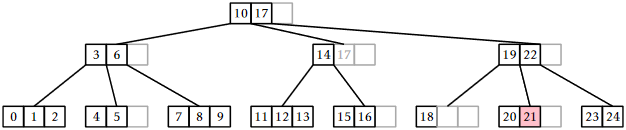
When an underflow occurs, $\mathtt{u}$ either borrows keys from, or is merged with, one of its siblings. If $\mathtt{u}$ is merged with a sibling, then $\mathtt{u}$'s parent will now have one less child and one less key, which can cause $\mathtt{u}$'s parent to underflow; this is again corrected by borrowing or merging, but merging may cause $\mathtt{u}$'s grandparent to underflow. This process works its way back up to the root until there is no more underflow or until the root has its last two children merged into a single child. When the latter case occurs, the root is removed and its lone child becomes the new root.

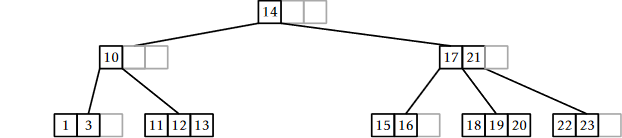
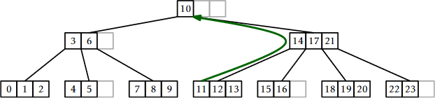
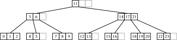
Next we delve into the details of how each of these steps is implemented. The first job of the $\mathtt{remove(x)}$ method is to find the element $\mathtt{x}$ that should be removed. If $\mathtt{x}$ is found in a leaf, then $\mathtt{x}$ is removed from this leaf. Otherwise, if $\mathtt{x}$ is found at $\texttt{u.keys[i]}$ for some internal node, $\mathtt{u}$, then the algorithm removes the smallest value, $\mathtt{x'}$, in the subtree rooted at $\mathtt{u.children[i+1]}$. The value $\mathtt{x'}$ is the smallest value stored in the BTree that is greater than $\mathtt{x}$. The value of $\mathtt{x'}$ is then used to replace $\mathtt{x}$ in $\texttt{u.keys[i]}$. This process is illustrated in Figure $\PageIndex{7}$.

Figure $\PageIndex{7}$: The $\mathtt{remove(x)}$ operation in a `BTree`. To remove the value $\mathtt{x}=10$ we replace it with the the value $\mathtt{x'}=11$ and remove 11 from the leaf that contains it.

The $\mathtt{removeRecursive(x,ui)}$ method is a recursive implementation of the preceding algorithm:

    boolean removeRecursive(T x, int ui) {
        if (ui < 0) return false;  // didn't find it
        Node u = bs.readBlock(ui);
        int i = findIt(u.keys, x);
        if (i < 0) { // found it
            i = -(i+1);
            if (u.isLeaf()) {
                u.remove(i);
            } else {
                u.keys[i] = removeSmallest(u.children[i+1]);
                checkUnderflow(u, i+1);
            }
            return true;  
        } else if (removeRecursive(x, u.children[i])) {
            checkUnderflow(u, i);
            return true;
        }
        return false;
    }
    T removeSmallest(int ui) {
        Node u = bs.readBlock(ui);
        if (u.isLeaf()) 
            return u.remove(0);
        T y = removeSmallest(u.children[0]);  
        checkUnderflow(u, 0);
        return y;
    }

Note that, after recursively removing the value $\mathtt{x}$ from the $\mathtt{i}$th child of $\mathtt{u}$, $\mathtt{removeRecursive(x,ui)}$ needs to ensure that this child still has at least $B-1$ keys. In the preceding code, this is done using a method called $\mathtt{checkUnderflow(x,i)}$, which checks for and corrects an underflow in the $\mathtt{i}$th child of $\mathtt{u}$. Let $\mathtt{w}$ be the $\mathtt{i}$th child of $\mathtt{u}$. If $\mathtt{w}$ has only $B-2$ keys, then this needs to be fixed. The fix requires using a sibling of $\mathtt{w}$. This can be either child $\mathtt{i}+1$ of $\mathtt{u}$ or child $\mathtt{i}-1$ of $\mathtt{u}$. We will usually use child $\mathtt{i}-1$ of $\mathtt{u}$, which is the sibling, $\mathtt{v}$, of $\mathtt{w}$ directly to its left. The only time this doesn't work is when $\mathtt{i}=0$, in which case we use the sibling directly to $\mathtt{w}$'s right.

    void checkUnderflow(Node u, int i) {
        if (u.children[i] < 0) return;
        if (i == 0) 
            checkUnderflowZero(u, i); // use u's right sibling
        else
            checkUnderflowNonZero(u,i);
    }

In the following, we focus on the case when $\mathtt{i}\neq 0$ so that any underflow at the $\mathtt{i}$th child of $\mathtt{u}$ will be corrected with the help of the $(\mathtt{i}-1)$st child of $\mathtt{u}$. The case $\mathtt{i}=0$ is similar and the details can be found in the accompanying source code.

To fix an underflow at node $\mathtt{w}$, we need to find more keys (and possibly also children), for $\mathtt{w}$. There are two ways to do this:

Borrowing:

If $\mathtt{w}$ has a sibling, $\mathtt{v}$, with more than $B-1$ keys, then $\mathtt{w}$ can borrow some keys (and possibly also children) from $\mathtt{v}$. More specifically, if $\mathtt{v}$ stores $\mathtt{size(v)}$ keys, then between them, $\mathtt{v}$ and $\mathtt{w}$ have a total of

\[ B-2 + \mathtt{size(w)} \ge 2B-2 \nonumber\]

keys. We can therefore shift keys from $\mathtt{v}$ to $\mathtt{w}$ so that each of $\mathtt{v}$ and $\mathtt{w}$ has at least $B-1$ keys. This process is illustrated in Figure $\PageIndex{8}$.

Figure $\PageIndex{8}$: If $\mathtt{v}$ has more than $B-1$ keys, then $\mathtt{w}$ can borrow keys from $\mathtt{v}$.

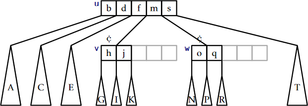
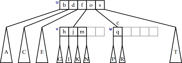
Merging:

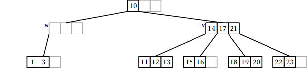
If $\mathtt{v}$ has only $B-1$ keys, we must do something more drastic, since $\mathtt{v}$ cannot afford to give any keys to $\mathtt{w}$. Therefore, we merge $\mathtt{v}$ and $\mathtt{w}$ as shown in Figure $\PageIndex{9}$. The merge operation is the opposite of the split operation. It takes two nodes that contain a total of $2B-3$ keys and merges them into a single node that contains $2B-2$ keys. (The additional key comes from the fact that, when we merge $\mathtt{v}$ and $\mathtt{w}$, their common parent, $\mathtt{u}$, now has one less child and therefore needs to give up one of its keys.)

    void checkUnderflowNonZero(Node u, int i) {
        Node w = bs.readBlock(u.children[i]);  // w is child of u
        if (w.size() < B-1) {  // underflow at w
            Node v = bs.readBlock(u.children[i-1]); // v left of w
            if (v.size() > B) {  // w can borrow from v
                shiftLR(u, i-1, v, w);
            } else { // v will absorb w
                merge(u, i-1, v, w);
            }
        }
    }
    void checkUnderflowZero(Node u, int i) {
        Node w = bs.readBlock(u.children[i]); // w is child of u
        if (w.size() < B-1) {  // underflow at w
            Node v = bs.readBlock(u.children[i+1]); // v right of w
            if (v.size() > B) { // w can borrow from v
                shiftRL(u, i, v, w);
            } else { // w will absorb w
                merge(u, i, w, v);
                u.children[i] = w.id;
            }
        }
    }

To summarize, the $\mathtt{remove(x)}$ method in a $B$-tree follows a root to leaf path, removes a key $\mathtt{x'}$ from a leaf, $\mathtt{u}$, and then performs zero or more merge operations involving $\mathtt{u}$ and its ancestors, and performs at most one borrowing operation. Since each merge and borrow operation involves modifying only three nodes, and only $O(\log_B \mathtt{n})$ of these operations occur, the entire process takes $O(\log_B \mathtt{n})$ time in the external memory model. Again, however, each merge and borrow operation takes $O(B)$ time in the word-RAM model, so (for now) the most we can say about the running time required by $\mathtt{remove(x)}$ in the word-RAM model is that it is $O(B\log_B \mathtt{n})$.

$\PageIndex{4}$ Amortized Analysis of $B$-Trees

Thus far, we have shown that

In the external memory model, the running time of $\mathtt{find(x)}$, $\mathtt{add(x)}$, and $\mathtt{remove(x)}$ in a $B$-tree is $O(\log_B \mathtt{n})$.
In the word-RAM model, the running time of $\mathtt{find(x)}$ is $O(\log \mathtt{n})$ and the running time of $\mathtt{add(x)}$ and $\mathtt{remove(x)}$ is $O(B\log \mathtt{n})$.

The following lemma shows that, so far, we have overestimated the number of merge and split operations performed by $B$-trees.

Lemma $\PageIndex{1}$.

Starting with an empty $B$-tree and performing any sequence of $m$ $\mathtt{add(x)}$ and $\mathtt{remove(x)}$ operations results in at most $3m/2$ splits, merges, and borrows being performed.

Proof. The proof of this has already been sketched in Section 9.3 for the special case in which $B=2$. The lemma can be proven using a credit scheme, in which

each split, merge, or borrow operation is paid for with two credits, i.e., a credit is removed each time one of these operations occurs; and
at most three credits are created during any $\mathtt{add(x)}$ or $\mathtt{remove(x)}$ operation.

Since at most $3m$ credits are ever created and each split, merge, and borrow is paid for with with two credits, it follows that at most $3m/2$ splits, merges, and borrows are performed. These credits are illustrated using the symbol in Figures $\PageIndex{4}$, $\PageIndex{8}$, and $\PageIndex{9}$.

To keep track of these credits the proof maintains the following credit invariant: Any non-root node with $B-1$ keys stores one credit and any node with $2B-1$ keys stores three credits. A node that stores at least $B$ keys and most $2B-2$ keys need not store any credits. What remains is to show that we can maintain the credit invariant and satisfy properties 1 and 2, above, during each $\mathtt{add(x)}$ and $\mathtt{remove(x)}$ operation.

$\qedsymbol$

$\PageIndex{4.0.1}$ Adding:

The $\mathtt{add(x)}$ method does not perform any merges or borrows, so we need only consider split operations that occur as a result of calls to $\mathtt{add(x)}$.

Each split operation occurs because a key is added to a node, $\mathtt{u}$, that already contains $2B-1$ keys. When this happens, $\mathtt{u}$ is split into two nodes, $\mathtt{u'}$ and $\mathtt{u''}$ having $B-1$ and $B$ keys, respectively. Prior to this operation, $\mathtt{u}$ was storing $2B-1$ keys, and hence three credits. Two of these credits can be used to pay for the split and the other credit can be given to $\mathtt{u'}$ (which has $B-1$ keys) to maintain the credit invariant. Therefore, we can pay for the split and maintain the credit invariant during any split.

The only other modification to nodes that occur during an $\mathtt{add(x)}$ operation happens after all splits, if any, are complete. This modification involves adding a new key to some node $\mathtt{u'}$. If, prior to this, $\mathtt{u'}$ had $2B-2$ children, then it now has $2B-1$ children and must therefore receive three credits. These are the only credits given out by the $\mathtt{add(x)}$ method.

$\PageIndex{4.0.2}$ Removing:

During a call to $\mathtt{remove(x)}$, zero or more merges occur and are possibly followed by a single borrow. Each merge occurs because two nodes, $\mathtt{v}$ and $\mathtt{w}$, each of which had exactly $B-1$ keys prior to calling $\mathtt{remove(x)}$ were merged into a single node with exactly $2B-2$ keys. Each such merge therefore frees up two credits that can be used to pay for the merge.

After any merges are performed, at most one borrow operation occurs, after which no further merges or borrows occur. This borrow operation only occurs if we remove a key from a leaf, $\mathtt{v}$, that has $B-1$ keys. The node $\mathtt{v}$ therefore has one credit, and this credit goes towards the cost of the borrow. This single credit is not enough to pay for the borrow, so we create one credit to complete the payment.

At this point, we have created one credit and we still need to show that the credit invariant can be maintained. In the worst case, $\mathtt{v}$'s sibling, $\mathtt{w}$, has exactly $B$ keys before the borrow so that, afterwards, both $\mathtt{v}$ and $\mathtt{w}$ have $B-1$ keys. This means that $\mathtt{v}$ and $\mathtt{w}$ each should be storing a credit when the operation is complete. Therefore, in this case, we create an additional two credits to give to $\mathtt{v}$ and $\mathtt{w}$. Since a borrow happens at most once during a $\mathtt{remove(x)}$ operation, this means that we create at most three credits, as required.

If the $\mathtt{remove(x)}$ operation does not include a borrow operation, this is because it finishes by removing a key from some node that, prior to the operation, had $B$ or more keys. In the worst case, this node had exactly $B$ keys, so that it now has $B-1$ keys and must be given one credit, which we create.

In either case--whether the removal finishes with a borrow operation or not--at most three credits need to be created during a call to $\mathtt{remove(x)}$ to maintain the credit invariant and pay for all borrows and merges that occur. This completes the proof of the lemma.

The purpose of Lemma $\PageIndex{1}$ is to show that, in the word-RAM model the cost of splits, merges and joins during a sequence of $m$ $\mathtt{add(x)}$ and $\mathtt{remove(x)}$ operations is only $O(Bm)$. That is, the amortized cost per operation is only $O(B)$, so the amortized cost of $\mathtt{add(x)}$ and $\mathtt{remove(x)}$ in the word-RAM model is $O(B+\log \mathtt{n})$. This is summarized by the following pair of theorems:

Theorem $\PageIndex{1}$. (External Memory $B$-Trees)

A BTree implements the SSet interface. In the external memory model, a BTree supports the operations $\mathtt{add(x)}$, $\mathtt{remove(x)}$, and $\mathtt{find(x)}$ in $O(\log_B \mathtt{n})$ time per operation.

Theorem $\PageIndex{2}$. (Word-RAM $B$-Trees)

A BTree implements the SSet interface. In the word-RAM model, and ignoring the cost of splits, merges, and borrows, a BTree supports the operations $\mathtt{add(x)}$, $\mathtt{remove(x)}$, and $\mathtt{find(x)}$ in $O(\log \mathtt{n})$ time per operation. Furthermore, beginning with an empty BTree, any sequence of $m$ $\mathtt{add(x)}$ and $\mathtt{remove(x)}$ operations results in a total of $O(Bm)$ time spent performing splits, merges, and borrows.

\(\PageIndex{1}\) Searching

\(\PageIndex{2}\) Addition

\(\PageIndex{3}\) Removal

\(\PageIndex{4}\) Amortized Analysis of \(B\)-Trees

\(\PageIndex{4.0.1}\) Adding:

\(\PageIndex{4.0.2}\) Removing: