7.1: Program Control Flow

This section demonstrates the use of the pc register to control the flow of program logic. To start, a simple function called increment is created, and this function is called from the main function. In the main function a variable called numToInc is created, and the increment function is called using the Branch-and-Link (bl) operator. The variable numToInc is passed to the function in r0, where it is incremented by 1 and returned back in r0.

This program is then run in gdb, and the value in the pc and lr registers follow to show how the pc is used to control program flow in this program.

7.1.1 main and increment functions

The program that will be used to illustrate program control flow is Program 9. The rest of this section will run this program in gdb and demonstrate how the pc and ldr registers are used in program control flow. To follow along with this discussion, enter this program into a file named incrementMain.s, compile and link the program, and begin to run the program, stopping it at the first line in the main method.

.global main 
main: 
    # Save return to os on stack 
    SUB sp, sp, #4 
    STR lr, [sp, #0] 
    
    # Prompt for and read input 
    LDR r0, =promptForNumber 
    BL printf 
    LDR r0, =inputNumber 
    LDR r1, =numToInc 
    BL scanf 
    
# Increment numToInc by calling increment     
    LDR r0, =numToInc 
    LDR r0, [r0, #0] 
    Bl increment 
    
# Printing the answer 
    MOV r1, r0 
    LDR r0, =formatOutput 
    BL printf 
    
# Return to the OS 
    LDR lr, [sp, #0] 
    ADD sp, sp, #4 
    MOV pc, lr 
    
.data 
    promptForNumber: .asciz "Enter the number you want to increment: \ n" 
    formatOutput: .asciz "\nThe input + 1 is %d\n" 
    inputNumber: .asciz "%d" 
    numToInc: .word 0 
#end main 
.text 
#function increment 
increment: 
    ADD r0, r0, #1 
    MOV pc, lr 
#end increment

9 Increment function

When the program reaches the breakpoint in the main, the screen should appear as follows:

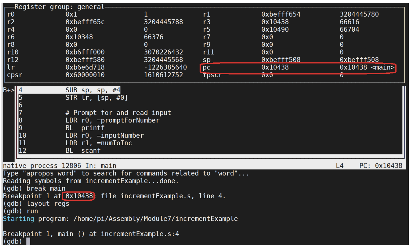
Figure 62: Start of the program to call the increment function

In this figure, the column to the left of the source program is the address in memory of that instruction. As this figure shows, the value in the pc register is the same as this address, and this shows that the pc register contains the current instruction that is being executed. By walking through the program using the next command, the next instruction is always 4 bytes away from the current instruction, and the pc is increased by 4. This is how the program runs sequential instructions in a program, by increasing the value of the pc register by 4 for each instruction.

Now set a break point at line 17, and continue running the program. Enter a value or 5 when the program pauses for input at the scanf statement. The program will stop at address 0x1045c, the bl instruction that references the increment function. This is shown in the following screen shot.

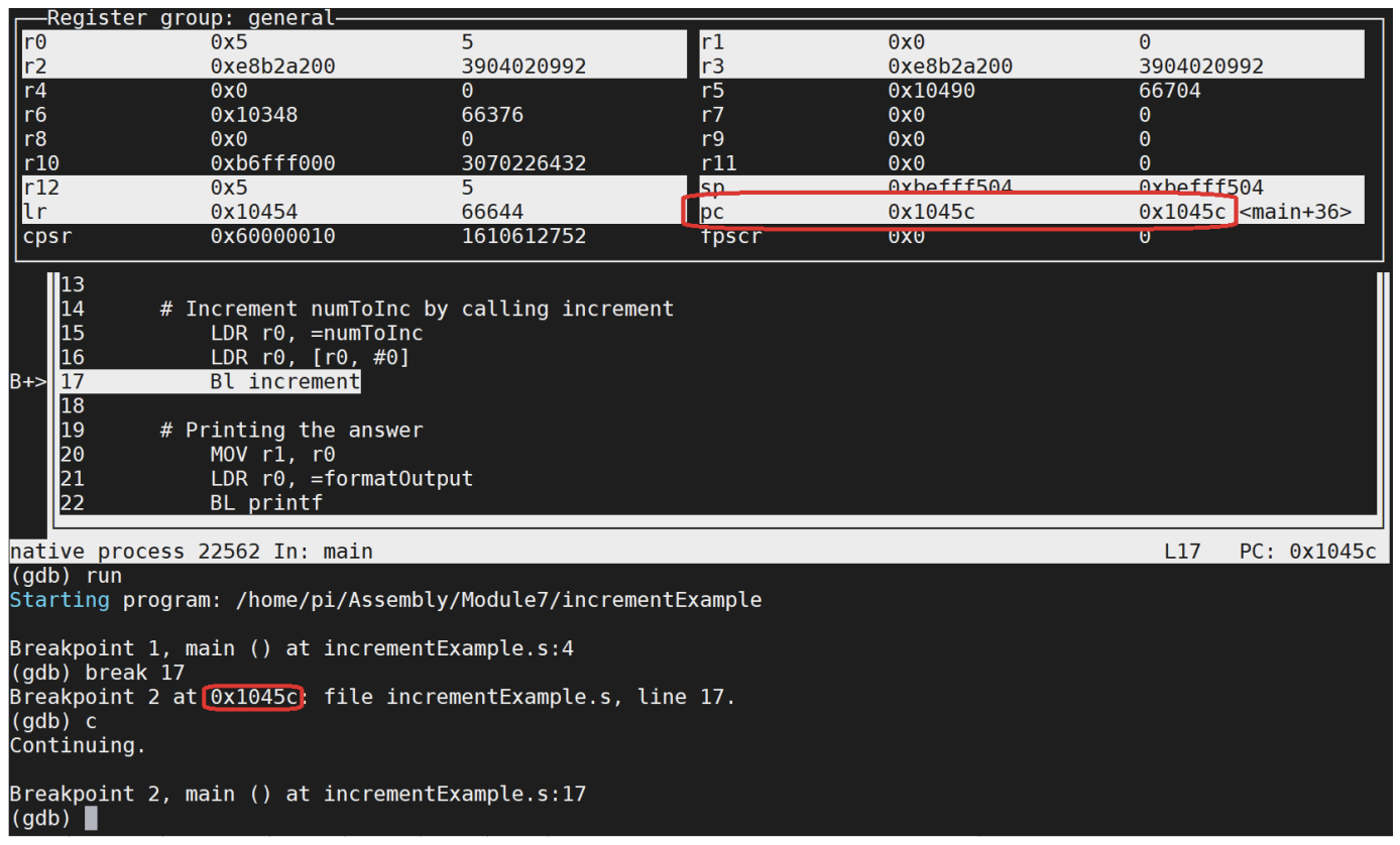
Figure 63: The branch and link command for the increment function

The branch instruction is used to cause the program to jump to an address other than the next sequential statement. This branch statement contains the value 0x10478, which is the address of the start of the increment function.

For now, think of the bl instruction as a function call. When calling a function, it is expected that when the function completes, it will return to the instruction after call to the function. In this case, that is the “MOV r1, r0” statement at address 0x10460. To allow the function to return to this address, the lr register is loaded with this address.

The step command (not the next command) in gdb steps into the method. Using step, step to the first instruction in increment. Notice the value in the pc is 0x10478, and the value in lr is 0x10460, as expected.

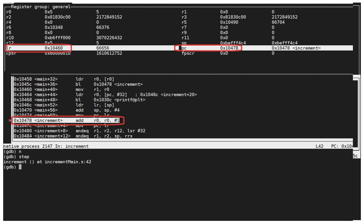
Figure 64: First statement when entering the increment function

The second instruction in the increment method is a “MOV pc, lr”, which moves the value in the lr (the return point in main) into the pc, which causes the program to return to the main. The screen after running this instruction should look as follows:

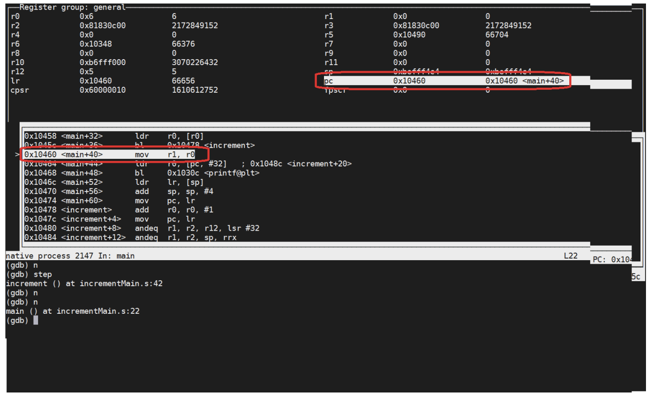
Figure 65: Return from the increment function

This shows the return from the function. This example is how the control of flow in a program is combined for a function using a combination of the pc and lr registers.

The important thing to remember about this section is that the pc controls program flow and is possibly the most important register in a computer.