14.4: Example

In this example, we will write a Fortran program that will request a count, generate count \((x,y)\) random points, and perform a Monte Carlo \(\pi\) estimation based on those points. All \(x\) and \(y\) values are between 0 and 1. The main routine will get the count and then use a subroutine to generate the random \((x,y)\) points and a function, to perform the Monte Carlo \(\pi\) estimation. For this example, the count should be between 100 and 1,000,000.

Understand the Problem

Based on the problem definition, the main routine that will read and verify the count value. If the count is not between 100 and 1,000,000, the routine will re-prompt until the correct input is provided. Once a valid count value is obtained, then the main will allocate the array and call the two subroutines.

The first subroutine will generate the random \((x,y)\) points and store them in an array. The second subroutine will perform the Monte Carlo \(\pi\) estimation.

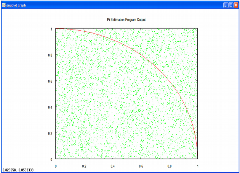
Monte Carlo methods are a class of computational algorithms that rely on repeated random sampling to compute their results. Suppose a square is centered on the origin of a Cartesian plane, and the square has sides of length 2. If we inscribe a circle in the square, it will have a diameter of length 2 and a radius of length 1. If we plot points within the upper right quadrant, the ratio between the points that land within the inscribed circle and the total points will be an estimation of \(\pi\).

\[ \textit{est }\pi = 4 \left( \frac{\text{samples inside circle}}{\text{total samples}} \right) \nonumber \]

As more samples are taken, the estimated value of \(\pi\) should approach the actual value of \(\pi\). The Pythagorean theorem can be used to determine the distance of the point from the origin. If this distance is less than the radius of the circle, then the point must be in the circle. Thus, if the square root of \((x^2 + y^2) < 1.0\), the random point is within the circle.

Finally, the figure we are discussing, a square centered on the origin with an inscribed circle is symmetric with respect to the quadrants of its Cartesian plane. This works well with the default random number generations of values between 0 and 1.

Create the Algorithm

The main routine will display an initial header, get and check the count value, and allocate the array. The program will need to ensure that the array is correctly allocated before proceeding. Then the program can generate the \((x,y)\) points. Based on the problem definition, each point should be between 0.0 and 1.0, which is provided by default by the Fortran random number generator. Next, the program can perform the Monte Carlo pi estimation. This will require the already populated \((x,y)\) points array and the count of points. Each point will be examined to determine the number of points that lie within the inscribed circle. The Pythagorean theorem allows us to determine the distance of the point from the origin (0.0,0.0). Thus, for each point, we will calculate the \(\sqrt{(x^2 + y^2)}\) and if the distance is less than the circle radius of 1.0, it will be counted as inside the circle.

Then, the estimated value of \(\pi\) can be calculated based on the formula:

\[ \textit{est } \pi = 4 \left( \frac{\text{samples inside circle}}{\text{total samples}} \right) \nonumber \]

When completed, the program will display the final results. The basic algorithm is as follows:

! declare variables
! display initial header
! prompt for and obtain count value
!     loop
!         prompt for count value
!         read count value
!         if count is correct, exit loop 
!         display error message
!     end loop
! allocate two dimension array
! generate points
!     loop count times
!         generate x and y values
!         place (x,y) values in array at appropriate index
!     end loop
! set count of samples inside circle = 0
!     loop count times
!         if [ sqrt (x(i)**2 + y(i)**2) < 1.0 ]
!             increment count of samples inside circle
!     end loop
! display results

For convenience, the steps are written as program comments.

Implement the Program

The following code results from the implementation of the preceding algorithm.

program piestimation

! declare variables
implicit none
integer :: count, alstat, i, incount
real :: x, y, pi_est, pt
real, allocatable, dimension(:,:) :: points

! display initial header
    write (*,'(/a/)') "Program Example – PI estimation."

! prompt for and obtain count value
    do
        ! prompt for count value
        write (*,'(a)', advance="no") &
            "Enter Count (100 - 1,000,000): "

        ! read count value
        read (*,*) count

        ! if count is correct, exit loop
        if ( count >= 100 .and. count <= 1000000 ) exit

        ! display error message
        write (*,'(a,a,/a)') "Error, count must be ", &
            "between 100 and 1,000,000.", &
            "Please re-enter." &
    end do

! allocate two dimension array
    allocate (points(count,2), stat=alstat)
    if (alstat /= 0 ) then
        write (*,'(a,a,/a)') "Error, unable to",
        " allocate memory.", "Program terminated."
        stop
    end if

! generate_points
    call random_seed()

    ! loop count times
    do i = 1, count
    
        ! generate x and y values
        call random_number(x)
        call random_number(y)
    
        ! place (x,y) values in array
        pts(i,1) = x
        pts(i,2) = y
    end do

! perform monte carlo estimation
    ! set count of samples inside circle = 0
    incount = 0
    
    ! loop count times
    do i = 1, count

    ! if[sqrt(x(i)2 +y(i)2)<1.0]
    !     increment count of samples inside circle

        pt = pts(i,1)**2 + pts(i,2)**2
        if (sqrt(pt) < 1.0) incount = incount + 1
    
    end do
    
    pi_est = 4.0 * real(incount) / real(count)

! display results
    write (*,'(a, f8.2)') "Count of points: ", count
    write (*,'(a, f8.2)') "Estimated PI value: ", pi_est

end program piestimation

The spacing and indentation are not required, but help to make the program more readable.

Test/Debug the Program

For this problem, the testing would involve executing the program using a series of different count values and ensure that the \(\pi\) estimate is reasonable and improves with higher count values.